github开源仓库
注意方向问题!意方向问题!方向问题!向问题!问题!题! ,以下所有分析皆是顺时针为正
单侧系统状态方程求解
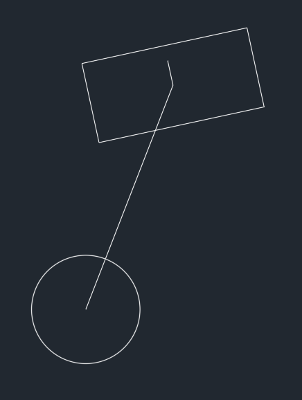
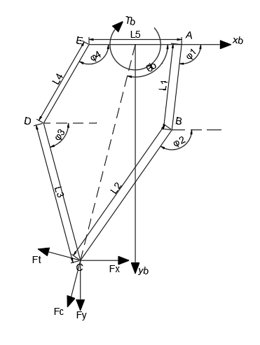
首先双轮足式机器人可以将模型化简为一个倒立摆模型,如下
分块开始分析
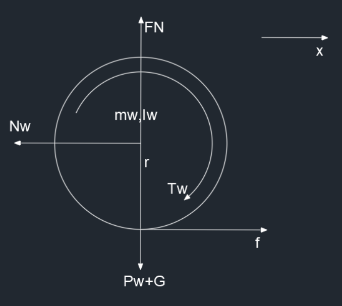
轮子
水平方向上
m w x ¨ = f − N w m_w\ddot{x}=f-N_w
m w x ¨ = f − N w
竖直方向上
F N = P w + G F_N=P_w+G
F N = P w + G
转矩
I w x ¨ r = T w − f r I_w\frac{\ddot{x}}{r}=T_w-fr
I w r x ¨ = T w − f r
联立消去 f f f
\ddot{x}=\frac{T_wr-N_wr^2}{I_w+m_wr^2}~~~~\textcircled{1}
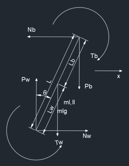
摆杆
水平方向上
m_l(\ddot{x}+\frac{\partial^2}{\partial t^2}L_w\sin\theta)=N_w-N_b~~~~\textcircled{2}
竖直方向上
m_l\frac{\partial^2}{\partial t^2}L_w\cos\theta=P_w-P_b-m_lg~~~~\textcircled{3}
转矩
I_l\ddot{\theta}=T_b-T_w+(P_bL_b+P_wL_w)\sin\theta-(N_bL_b+N_wL_w)\cos\theta~~~~\textcircled{4}
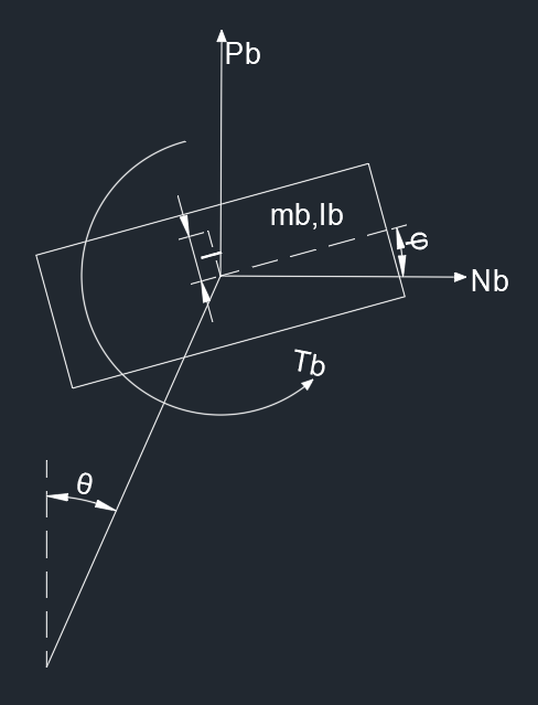
机体
水平方向上
m_b(\ddot{x}+\frac{\partial^2}{\partial t^2}L\sin\theta-\frac{\partial^2}{\partial t^2}l\sin\varphi)=N_b~~~~\textcircled{5}
竖直方向上
m_b(\frac{\partial^2}{\partial t^2}L\cos\theta+\frac{\partial^2}{\partial t^2}l\cos\varphi)=P_b-m_bg~~~~\textcircled{6}
转矩
I_b\ddot{\varphi}=T_b+N_bl\cos\varphi+P_bl\sin\varphi~~~~\textcircled{7}
根据上述得到的 \textcircled{2}\textcircled{3}\textcircled{5}\textcircled{6} 联立,得到中间变量 P w , N w , P b , N b P_w,N_w,P_b,N_b P w , N w , P b , N b
{ P w = m b ( ∂ 2 ∂ t 2 L cos θ + ∂ 2 ∂ t 2 l cos φ ) + m b g + m l ∂ 2 ∂ t 2 L w cos θ + m l g N w = m l ( x ¨ + ∂ 2 ∂ t 2 L w sin θ ) + m b ( x ¨ + ∂ 2 ∂ t 2 L sin θ − ∂ 2 ∂ t 2 l sin φ ) P b = m b ( ∂ 2 ∂ t 2 L cos θ + ∂ 2 ∂ t 2 l cos φ ) + m b g N b = m b ( x ¨ + ∂ 2 ∂ t 2 L sin θ − ∂ 2 ∂ t 2 l sin φ ) \left\{\begin{aligned}&P_w=m_b(\frac{\partial^2}{\partial t^2}L\cos\theta+\frac{\partial^2}{\partial t^2}l\cos\varphi)+m_bg+m_l\frac{\partial^2}{\partial t^2}L_w\cos\theta+m_lg\\&N_w=m_l(\ddot{x}+\frac{\partial^2}{\partial t^2}L_w\sin\theta)+m_b(\ddot{x}+\frac{\partial^2}{\partial t^2}L\sin\theta-\frac{\partial^2}{\partial t^2}l\sin\varphi)\\&P_b=m_b(\frac{\partial^2}{\partial t^2}L\cos\theta+\frac{\partial^2}{\partial t^2}l\cos\varphi)+m_bg\\&N_b=m_b(\ddot{x}+\frac{\partial^2}{\partial t^2}L\sin\theta-\frac{\partial^2}{\partial t^2}l\sin\varphi)\end{aligned}\right.
⎩ ⎪ ⎪ ⎪ ⎪ ⎪ ⎪ ⎪ ⎪ ⎪ ⎪ ⎪ ⎨ ⎪ ⎪ ⎪ ⎪ ⎪ ⎪ ⎪ ⎪ ⎪ ⎪ ⎪ ⎧ P w = m b ( ∂ t 2 ∂ 2 L cos θ + ∂ t 2 ∂ 2 l cos φ ) + m b g + m l ∂ t 2 ∂ 2 L w cos θ + m l g N w = m l ( x ¨ + ∂ t 2 ∂ 2 L w sin θ ) + m b ( x ¨ + ∂ t 2 ∂ 2 L sin θ − ∂ t 2 ∂ 2 l sin φ ) P b = m b ( ∂ t 2 ∂ 2 L cos θ + ∂ t 2 ∂ 2 l cos φ ) + m b g N b = m b ( x ¨ + ∂ t 2 ∂ 2 L sin θ − ∂ t 2 ∂ 2 l sin φ )
带入 \textcircled{1}\textcircled{4}\textcircled{7} 中,并且利用 matlab 的符号求解工具解。设定
X = [ θ θ ˙ x x ˙ φ φ ˙ ] U = [ T w T b ] X=\begin{bmatrix}\theta\\\dot{\theta}\\x\\\dot{x}\\\varphi\\\dot\varphi\end{bmatrix}\\U=\begin{bmatrix}T_w\\T_b\end{bmatrix}
X = ⎣ ⎢ ⎢ ⎢ ⎢ ⎢ ⎢ ⎢ ⎡ θ θ ˙ x x ˙ φ φ ˙ ⎦ ⎥ ⎥ ⎥ ⎥ ⎥ ⎥ ⎥ ⎤ U = [ T w T b ]
最终求解对应的雅各比矩阵,就是 A 和 B
1
2
3
4
5
6
7
8
9
10
11
12
13
14
15
16
17
18
19
20
21
22
23
24
25
26
27
28
29
30
31
32
33
34
clc clear syms x(t) theta(t) phi(t) syms Tw Tb Pw Pb Nw Nb syms x_ddot theta_ddot phi_ddot x_dot theta_dot phi_dot syms mw R Iw mb Ib_y g Ic_z R_l l ml syms L Il Lw Lb func1 = [ml * diff(diff(x + Lw * sin (theta), t), t) == Nw - Nb; ml * diff(diff(Lw * cos (theta), t), t) == Pw - Pb - ml * g; mb * diff(diff(x + L * sin (theta) - l * sin (phi), t), t) == Nb; mb * diff(diff(L * cos (theta) + l * cos (phi), t), t) == Pb - mb * g; ]; [Pw, Pb, Nw, Nb] = solve(func1, [Pw, Pb, Nw, Nb]); func2 = [diff(diff(x, t), t) == (Tw * R - Nw * R * R) / (Iw + mw * R * R); Il * diff(diff(theta, t), t) == Tb - Tw + (Pb * Lb + Pw * Lw) * sin (theta) - (Nb * Lb + Nw * Lw) * cos (theta); Ib_y * diff(diff(phi, t), t) == Tb + Nb * l * cos (phi) + Pb * l * sin (phi);]; func2 = subs(func2, ... [diff(diff(x, t), t), diff(diff(theta, t), t), diff(diff(phi, t), t), diff(x, t), diff(theta, t), diff(phi, t)], ... [x_ddot, theta_ddot, phi_ddot, x_dot, theta_dot, phi_dot]); [x_ddot, theta_ddot, phi_ddot] = solve(func2, [x_ddot theta_ddot phi_ddot]); X = [theta(t); theta_dot; x(t); x_dot; phi(t); phi_dot]; u = [Tw; Tb]; X_dot = [theta_dot; theta_ddot; x_dot; x_ddot; phi_dot; phi_ddot]; A = jacobian(X_dot, X); B = jacobian(X_dot, u); A = subs(A, [x_dot, theta(t), theta_dot, phi(t), phi_dot, Tw, Tb], zeros (1 ,7 )) B = subs(B, [x_dot, theta(t), theta_dot, phi(t), phi_dot, Tw, Tb], zeros (1 ,7 ))
最终得到结果,有点复杂,之前那个是解算出错了 T_T
这就是系统状态空间方程
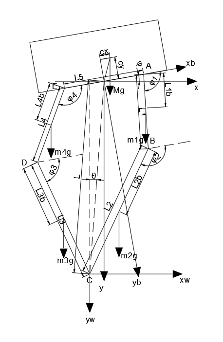
腿部质心拟合
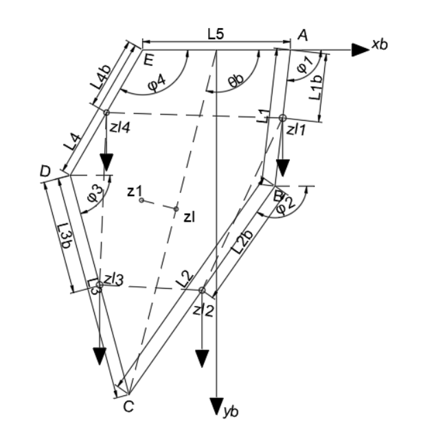
由于在分析和设计控制器的过程中,机器人的腿部连杆需要简化为一个直杆,所以就需要将原来的腿部连杆的转动惯量和质心拟合到虚拟的杆上,如图所示
这里使用机体坐标系,计算可以得到每个杆的坐标位置,这里借用一下下面的五连杆求解结果,根据得到的 φ 2 \varphi_2 φ 2 φ 3 \varphi_3 φ 3
Z l 1 = [ l 5 2 + l 1 b cos φ 1 l 1 b sin φ 1 ] Z l 2 = [ l 5 2 + l 1 cos φ 1 + l 2 b cos φ 2 l 1 sin φ 1 + l 2 b sin φ 2 ] Z l 3 = [ − l 5 2 + l 4 cos φ 4 + l 3 b cos φ 3 l 4 sin φ 4 + l 3 b sin φ 3 ] Z l 4 = [ − l 5 2 + l 4 b cos φ 4 l 4 b sin φ 4 ] Z_{l_1}=\begin{bmatrix}\frac{l_5}{2}+l_{1b}\cos\varphi_1\\l_{1b}\sin\varphi_1\end{bmatrix}\\Z_{l_2}=\begin{bmatrix}\frac{l_5}{2}+l_1\cos\varphi_1+l_{2b}\cos\varphi_2\\l_1\sin\varphi_1+l_{2b}\sin\varphi_2\end{bmatrix}\\Z_{l_3}=\begin{bmatrix}-\frac{l_5}{2}+l_4\cos\varphi_4+l_{3b}\cos\varphi_3\\l_4\sin\varphi_4+l_{3b}\sin\varphi_3\end{bmatrix}\\Z_{l_4}=\begin{bmatrix}-\frac{l_5}{2}+l_{4b}\cos\varphi_4\\l_{4b}\sin\varphi_4\end{bmatrix}
Z l 1 = [ 2 l 5 + l 1 b cos φ 1 l 1 b sin φ 1 ] Z l 2 = [ 2 l 5 + l 1 cos φ 1 + l 2 b cos φ 2 l 1 sin φ 1 + l 2 b sin φ 2 ] Z l 3 = [ − 2 l 5 + l 4 cos φ 4 + l 3 b cos φ 3 l 4 sin φ 4 + l 3 b sin φ 3 ] Z l 4 = [ − 2 l 5 + l 4 b cos φ 4 l 4 b sin φ 4 ]
根据如下式子求解出四个连杆的质心位置为 Z 1 Z_1 Z 1
( m 1 + m 2 + m 3 + m 4 ) Z 1 = m 1 Z l 1 x + m 2 Z l 2 x + m 3 Z l 3 x + m 4 Z l 4 x (m_1+m_2+m_3+m_4)Z_1=m_1Z_{l_1x}+m_2Z_{l_2x}+m_3Z_{l_3x}+m_4Z_{l_4x}
( m 1 + m 2 + m 3 + m 4 ) Z 1 = m 1 Z l 1 x + m 2 Z l 2 x + m 3 Z l 3 x + m 4 Z l 4 x
求解出的连杆质心之后,还要将其映射到虚拟杆上,这里选择直接对虚拟杆作垂线
( Z 1 y − Z l y Z 1 x − Z l x ) ( C y − 0 C x − 0 ) = − 1 C y − Z l y C x − Z l x = C y − 0 C x − 0 (\frac{Z_{1y}-Z_{ly}}{Z_{1x}-Z_{lx}})(\frac{C_y-0}{C_x-0})=-1\\\frac{C_y-Z_{ly}}{C_x-Z_{lx}}=\frac{C_y-0}{C_x-0}
( Z 1 x − Z l x Z 1 y − Z l y ) ( C x − 0 C y − 0 ) = − 1 C x − Z l x C y − Z l y = C x − 0 C y − 0
最终求解得到虚拟杆的质心 Z l Z_l Z l
I l = ∑ i 4 I i + m i ( Z l − Z l i ) T ( Z l − Z l i ) I_l=\sum_i^4I_i+m_i(Z_l-Z_{l_i})^T(Z_l-Z_{l_i})
I l = i ∑ 4 I i + m i ( Z l − Z l i ) T ( Z l − Z l i )
同时也可以计算出所需要的 L w L_w L w L b L_b L b
L w = ( Z l − C ) T ( Z l − C ) L b = ( Z l − 0 ) T ( Z l − 0 ) L_w=\sqrt{(Z_l-C)^T(Z_l-C)}\\L_b=\sqrt{(Z_l-0)^T(Z_l-0)}
L w = ( Z l − C ) T ( Z l − C ) L b = ( Z l − 0 ) T ( Z l − 0 )
LQR 控制器
首先是 LQR 控制器。是一个比较常用的控制器,设计起来也比较简单。
推导过程与一般的 LQR 无异,所以直接调用 matlab 函数来求得对应的 K,最终需要拟合出一个 K 关于杆长的函数
1 2 3 4 5 6 7 C = eye (6 ); D = zeros (6 ,2 ); Q = diag ([100 100 100 10 5000 1 ]); R = diag ([1 0.25 ]); sys = ss(A, B, C, D); KLQR = lqr(sys, Q, R);
其中的 Q 和 R 就是系统状态与系统输入的权重,越大表示越在意
最终需要将控制器反馈增益矩阵拟合为关于杆长的一元三次方程,具体的拟合代码为
1
2
3
4
5
6
7
8
9
10
11
12
13
14
15
16
17
18
19
20
21
22
23
24
25
26
27
28
29
30
31
32
33
34
35
36
37
38
39
40
41
42
43
44
45
46
47
48
49
50
51
52
53
54
55
56
57
58
59
60
61
62
63
64
65
66
67
68
69
70
71
72
73
74
75
76
77
78
79
80
81
82
83
84
85
86
87
88
89
90
91
92
93
94
95
96
97
98
99
100
101
102
103
104
105
106
107
108
clc clear syms x(t) theta(t) phi(t) syms Tw Tb Pw Pb Nw Nb syms x_ddot theta_ddot phi_ddot x_dot theta_dot phi_dot syms L Il Lw Lb ml mw = 0.77115000 * 2 ; R = 0.1 ; Iw = 0.00379267 * 2 ; mb = 5.4940204 ; Ib_y = 0.05019911 ; g = 9.81 ; Ic_z = 0.37248874 ; R_l = 0.482000001 ; l = -0.02011323 ; func1 = [ml * diff(diff(x + Lw * sin (theta), t), t) == Nw - Nb; ml * diff(diff(Lw * cos (theta), t), t) == Pw - Pb - ml * g; mb * diff(diff(x + L * sin (theta) - l * sin (phi), t), t) == Nb; mb * diff(diff(L * cos (theta) + l * cos (phi), t), t) == Pb - mb * g; ]; [Pw, Pb, Nw, Nb] = solve(func1, [Pw, Pb, Nw, Nb]); func2 = [diff(diff(x, t), t) == (Tw * R - Nw * R * R) / (Iw + mw * R * R); Il * diff(diff(theta, t), t) == Tb - Tw + (Pb * Lb + Pw * Lw) * sin (theta) - (Nb * Lb + Nw * Lw) * cos (theta); Ib_y * diff(diff(phi, t), t) == Tb + Nb * l * cos (phi) + Pb * l * sin (phi);]; func2 = subs(func2, ... [diff(diff(x, t), t), diff(diff(theta, t), t), diff(diff(phi, t), t), diff(x, t), diff(theta, t), diff(phi, t)], ... [x_ddot, theta_ddot, phi_ddot, x_dot, theta_dot, phi_dot]); [x_ddot, theta_ddot, phi_ddot] = solve(func2, [x_ddot theta_ddot phi_ddot]); X = [theta(t); theta_dot; x(t); x_dot; phi(t); phi_dot]; u = [Tw; Tb]; X_dot = [theta_dot; theta_ddot; x_dot; x_ddot; phi_dot; phi_ddot]; A = jacobian(X_dot, X); B = jacobian(X_dot, u); A = subs(A, [x_dot, theta(t), theta_dot, phi(t), phi_dot, Tw, Tb], zeros (1 ,7 )); B = subs(B, [x_dot, theta(t), theta_dot, phi(t), phi_dot, Tw, Tb], zeros (1 ,7 )); minangle4 = -15 ; maxangle4 = 79 ; steps = 0.2 ; numsize = (maxangle4 - minangle4) / steps + 1 ; K_vals = zeros (numsize, 2 , 6 ); L_vals = zeros (numsize, 1 ); angle1_vals = zeros (numsize, 1 ); angle4_vals = zeros (numsize, 1 ); a = 1 ; for angle4 = minangle4 : steps : maxangle4 angle1 = 180 - angle4; [valml, valIl, valL, valLw, valLb] = GetLegBaryCenter(angle1, angle4, 0 ); valA = subs(A, [ml, Il, L, Lw, Lb], [2 * valml, 2 * valIl, valL, valLw, valLb]); valB = subs(B, [ml, Il, L, Lw, Lb], [2 * valml, 2 * valIl, valL, valLw, valLb]); valA = double(valA); valB = double(valB); if (rank(ctrb(valA, valB)) == size (valA, 1 )) disp ('系统可控' ) else disp ('系统不可控' ) K = 0 ; return end C = eye (6 ); D = zeros (6 ,2 ); Q = diag ([1 1 100 80 30 1 ]); R = diag ([1 0.25 ]); sys = ss(valA, valB, C, D); KLQR = lqr(sys, Q, R); K_vals(a, :, :) = KLQR; L_vals(a) = valL; a = a + 1 ; end K_coefficient = []; for i = 1 :1 :2 for j = 1 : 1 : 6 column_K = K_vals(:,i , j ); K_coefficient = [K_coefficient; polyfit(L_vals, column_K, 3 )]; end end disp (K_coefficient)Kk11 = polyfit(L_ranges, K_vals(:, 1 , 1 )', 3 ); Kk12 = polyfit(L_ranges, K_vals(:, 1 , 2 )', 3 ); Kk13 = polyfit(L_ranges, K_vals(:, 1 , 3 )', 3 ); Kk14 = polyfit(L_ranges, K_vals(:, 1 , 4 )', 3 ); Kk15 = polyfit(L_ranges, K_vals(:, 1 , 5 )', 3 ); Kk16 = polyfit(L_ranges, K_vals(:, 1 , 6 )', 3 ); Kk21 = polyfit(L_ranges, K_vals(:, 2 , 1 )', 3 ); Kk22 = polyfit(L_ranges, K_vals(:, 2 , 2 )', 3 ); Kk23 = polyfit(L_ranges, K_vals(:, 2 , 3 )', 3 ); Kk24 = polyfit(L_ranges, K_vals(:, 2 , 4 )', 3 ); Kk25 = polyfit(L_ranges, K_vals(:, 2 , 5 )', 3 ); Kk26 = polyfit(L_ranges, K_vals(:, 2 , 6 )', 3 ); Kk = [Kk11;Kk12; Kk13; Kk14; Kk15; Kk16; Kk21; Kk22; Kk23; Kk24; Kk25; Kk26];
可以使用 Curve Fitting Toolbox,能清楚的可视化数据的变化情况
整体状态空间方程
与单侧的平衡状态空间方程的建立基本上是一致的,但是需要同时注意左右两侧,并且还有一些整体机器人的分析。
轮子
左侧
水平方向上
m_{w,l}\ddot{x}_l=f_l-N_{w,l}~~~~\textcircled{1}
竖直方向上
F_{N,l}=P_{w,l}+G~~~~\textcircled{2}
转矩
I_{w,l}\frac{\ddot{x}_l}{R}=T_{w,l}-f_lR~~~~\textcircled{3}
右侧
水平方向上
m_{w,r}\ddot{x}_r=f_r-N_{w,r}~~~~\textcircled{4}
竖直方向上
F_{N,r}=P_{w,r}+G~~~~\textcircled{5}
转矩
I_{w,r}\frac{\ddot{x}_r}{R}=T_{w,r}-f_rR~~~~\textcircled{6}
摆杆
左侧
水平方向上
m_{l,l}(\ddot{x}_l+\frac{\partial^2}{\partial t^2}L_{w,l}\sin\theta_l)=N_{w,l}-N_{b,l}~~~~\textcircled{7}
竖直方向上
m_{l,l}\frac{\partial^2}{\partial t^2}L_{w,l}\cos\theta_l=P_{w,l}-P_{b,l}-m_{l,l}g~~~~\textcircled{8}
转矩
I_{l,l}\ddot{\theta_l}=T_{b,l}-T_{w,l}+(P_{b,l}L_{b,l}+P_{w,l}L_{w,l})\sin\theta_l-(N_{b,l}L_{b,l}+N_{w,l}L_{w,l})\cos\theta_l~~~~\textcircled{9}
右侧
水平方向上
m_{l,r}(\ddot{x}_r+\frac{\partial^2}{\partial t^2}L_{w,r}\sin\theta_r)=N_{w,r}-N_{b,r}~~~~\textcircled{10}
竖直方向上
m_{l,r}\frac{\partial^2}{\partial t^2}L_{w,r}\cos\theta_r=P_{w,r}-P_{b,r}-m_{l,r}g~~~~\textcircled{11}
转矩
I_{l,r}\ddot{\theta_r}=T_{b,r}-T_{w,r}+(P_{b,r}L_{b,r}+P_{w,r}L_{w,r})\sin\theta_r-(N_{b,r}L_{b,r}+N_{w,r}L_{w,r})\cos\theta_r~~~~\textcircled{12}
机体
水平方向上
m_b\frac{\partial^2}{\partial t^2}[\frac{1}{2}({x}_l+L_l\sin\theta_l+{x}_r+L_r\sin\theta_r)-l\sin\varphi]=N_{b,l}+N_{b,r}~~~~\textcircled{13}
竖直方向上
m_b\frac{\partial^2}{\partial t^2}[\frac{1}{2}(L_l\cos\theta_l+L_r\cos\theta_r)+l\cos\varphi]=P_{b,l}+P_{b,r}-m_bg~~~~\textcircled{14}
转矩
I_b\ddot{\varphi}=T_{b,l}+T_{b,r}+(N_{b,l}+N_{b,r})l\cos\varphi+(P_{b,l}+P_{b,r})l\sin\varphi~~~~\textcircled{15}
假设机体两侧支持力大小一致
P_{b,l}=P_{b,r}~~~~\textcircled{16}
整车的航向角
I_{c,z}\ddot{\psi}=(f_r-f_l)R_l~~~~\textcircled{17}\\\ddot{\psi}=\frac{\partial^2}{\partial t^2}\frac{(x_r+L_r\sin\theta_r-x_l-L_l\sin\theta_l)}{2R_l}~~~~\textcircled{18}
对上述中所有式子进行机体倾角进行小角度近似,然后利用其中的 \textcircled{1}\textcircled{4}\textcircled{7}\textcircled{8}\textcircled{10}\textcircled{11}\textcircled{13}\textcircled{14}\textcircled{16}\textcircled{17} 式求解出中间变量 P w , l , N w , l , P b , l , N b , l , P w , r , N w , r , P b , r , N b , r , f l , f r P_{w,l},N_{w,l},P_{b,l},N_{b,l},P_{w,r},N_{w,r},P_{b,r},N_{b,r},f_l,f_r P w , l , N w , l , P b , l , N b , l , P w , r , N w , r , P b , r , N b , r , f l , f r θ l , θ r , ϕ \theta_l, \theta_r, \phi θ l , θ r , ϕ
然后利用其中的 \textcircled{3}\textcircled{6}\textcircled{9}\textcircled{12}\textcircled{15} 来求解 x ¨ l , x ¨ r , θ ¨ l , θ ¨ r , φ ¨ \ddot{x}_l, \ddot{x}_r, \ddot{\theta}_l,\ddot{\theta}_r,\ddot{\varphi} x ¨ l , x ¨ r , θ ¨ l , θ ¨ r , φ ¨ \textcircled{18} 可以得到 ψ ¨ \ddot{\psi} ψ ¨
定义车子移动距离的表达式
s = x l + x r 2 ⇓ s ¨ = x ¨ l + x ¨ r 2 s=\frac{x_l+x_r}{2}\\\Downarrow\\\ddot{s}=\frac{\ddot{x}_l+\ddot{x}_r}{2}
s = 2 x l + x r ⇓ s ¨ = 2 x ¨ l + x ¨ r
可以得到 s ¨ \ddot{s} s ¨
定义
X = [ s s ˙ ψ ψ ˙ θ l θ ˙ l θ r θ ˙ r φ φ ˙ ] U = [ T w , l T w , r T b , l T b , r ] X=\begin{bmatrix}s\\\dot{s}\\\psi\\\dot{\psi}\\\theta_l\\\dot{\theta}_l\\\theta_r\\\dot{\theta}_r\\\varphi\\\dot{\varphi}\end{bmatrix}\\U=\begin{bmatrix}T_{w,l}\\T_{w,r}\\T_{b,l}\\T_{b,r}\end{bmatrix}
X = ⎣ ⎢ ⎢ ⎢ ⎢ ⎢ ⎢ ⎢ ⎢ ⎢ ⎢ ⎢ ⎢ ⎢ ⎢ ⎢ ⎡ s s ˙ ψ ψ ˙ θ l θ ˙ l θ r θ ˙ r φ φ ˙ ⎦ ⎥ ⎥ ⎥ ⎥ ⎥ ⎥ ⎥ ⎥ ⎥ ⎥ ⎥ ⎥ ⎥ ⎥ ⎥ ⎤ U = ⎣ ⎢ ⎢ ⎢ ⎡ T w , l T w , r T b , l T b , r ⎦ ⎥ ⎥ ⎥ ⎤
其中 ψ \psi ψ φ \varphi φ
最终可以得到系统状态方程的表达式。这里就不列出来了,太复杂了。直接上代码
电脑毁灭者——未进行小角度近似
1
2
3
4
5
6
7
8
9
10
11
12
13
14
15
16
17
18
19
20
21
22
23
24
25
26
27
28
29
30
31
32
33
34
35
36
37
38
39
40
41
42
43
44
45
46
47
48
49
50
51
52
53
54
55
56
57
58
59
60
61
62
63
64
65
66
67
68
69
70
71
72
73
74
75
76
77
78
79
80
81
82
83
84
85
86
87
88
89
90
91
92
93
94
95
96
97
98
99
100
101
102
103
104
105
106
107
108
109
110
111
112
113
114
115
116
117
118
119
120
121
122
123
124
125
126
127
128
129
130
131
132
133
134
135
136
137
138
139
140
141
142
143
144
145
146
147
148
149
150
151
152
153
154
155
156
157
158
159
160
161
162
163
164
165
166
167
168
169
170
171
172
173
174
clc clear syms theta_l(t) theta_r(t) phi(t) s(t) psi (t) x_l(t) x_r(t) syms mw_l mw_r f_l f_r Nw_l Nw_r Pw_l Pw_r Iw_l Iw_r R Tw_l Tw_r syms ml_l ml_r Il_l Il_r Lw_l Lw_r Lb_l Lb_r L_l L_r syms mb Ib_x Ib_y Ib_z l Tb_l Tb_r Nb_l Nb_r Pb_l Pb_r syms g syms wb_z R_l syms x_l_dot x_r_dot theta_l_dot theta_r_dot phi_dot s_dot psi_dot syms x_l_ddot x_r_ddot theta_l_ddot theta_r_ddot phi_ddot s_ddot psi_ddot xw_l = x_l; xw_r = x_r; FrontW_l = mw_l * diff(diff(xw_l, t), t) == f_l - Nw_l; TorqueW_l = Iw_l * diff(diff(xw_l, t), t) / R == Tw_l - f_l * R; FrontW_r = mw_r * diff(diff(xw_r, t), t) == f_r - Nw_r; TorqueW_r = Iw_r * diff(diff(xw_r, t), t) / R == Tw_r - f_r * R; xl_l = x_l + Lw_l * sin (theta_l); xl_r = x_r + Lw_r * sin (theta_r); yl_l = Lw_l * cos (theta_l); yl_r = Lw_r * cos (theta_r); FrontL_l = ml_l * diff(diff(xl_l, t), t) == Nw_l - Nb_l; UpL_l = ml_l * diff(diff(yl_l, t), t) == Pw_l - Pb_l - ml_l * g; TorqueL_l = Il_l * diff(diff(theta_l, t), t) == Tb_l - Tw_l + (Pb_l * Lb_l + Pw_l * Lw_l) * sin (theta_l) - (Nb_l * Lb_l + Nw_l * Lw_l) * cos (theta_l); FrontL_r = ml_r * diff(diff(xl_r, t), t) == Nw_r - Nb_r; UpL_r = ml_r * diff(diff(yl_r, t), t) == Pw_r - Pb_r - ml_r * g; TorqueL_r = Il_r * diff(diff(theta_r, t), t) == Tb_r - Tw_r + (Pb_r * Lb_r + Pw_r * Lw_r) * sin (theta_r) - (Nb_r * Lb_r + Nw_r * Lw_r) * cos (theta_r); xb = 0.5 * (x_l + L_l * sin (theta_l) + x_r + L_r * sin (theta_r)) - l * sin (phi); yb = 0.5 * (L_l * cos (theta_l) + L_r * cos (theta_r)) + l * cos (phi); FrontB = mb * diff(diff(xb, t), t) == Nb_l + Nb_r; UpB = mb * diff(diff(yb, t), t) == Pb_l + Pb_r - mb * g; TorqueB = Ib_y * diff(diff(phi, t), t) == (Tb_l + Tb_r) + (Nb_l + Nb_r) * l * cos (phi) + (Pb_l + Pb_r) * l * sin (phi); ForceEqual = Pw_l == Pw_r; psi_ = (x_r - x_l + L_r * sin (theta_r) - L_l * sin (theta_l)) / 2 / R_l; WholeTurn = wb_z * diff(diff(psi_, t), t) == (f_r - f_l) * R_l; func1 = [FrontW_l; FrontW_r; FrontL_l; FrontL_r; UpL_l; UpL_r; FrontB; UpB; ForceEqual; WholeTurn]; [valPw_l, valPw_r, valNw_l, valNw_r, valPb_l, valPb_r, valNb_l, valNb_r, valf_l, valf_r] = solve(func1, [Pw_l, Pw_r, Nw_l, Nw_r, Pb_l, Pb_r, Nb_l, Nb_r, f_l, f_r]); func2 = [TorqueW_l; TorqueW_r; TorqueL_l; TorqueL_r; TorqueB]; func2 = subs(func2, ... [Pw_l, Pw_r, Nw_l, Nw_r, Pb_l, Pb_r, Nb_l, Nb_r, f_l, f_r], ... [valPw_l, valPw_r, valNw_l, valNw_r, valPb_l, valPb_r, valNb_l, valNb_r, valf_l, valf_r]); func2 = subs(func2, ... [diff(diff(x_l, t), t), diff(diff(x_r, t), t), diff(diff(theta_l, t), t), diff(diff(theta_r, t), t), diff(diff(phi, t), t), diff(x_l, t), diff(x_r, t), diff(theta_l, t), diff(theta_r, t), diff(phi, t)], ... [x_l_ddot, x_r_ddot, theta_l_ddot, theta_r_ddot, phi_ddot, x_l_dot, x_r_dot, theta_l_dot, theta_r_dot, phi_dot]); [x_l_ddot, x_r_ddot, theta_l_ddot, theta_r_ddot, phi_ddot] = vpasolve(func2, [x_l_ddot, x_r_ddot, theta_l_ddot, theta_r_ddot, phi_ddot]); X_dot = [x_l_dot, x_l_ddot, x_r_dot, x_r_ddot, theta_l_dot, theta_l_ddot, theta_r_dot, theta_r_ddot, phi_dot, phi_ddot]; X = [x_l, x_l_dot, x_r, x_r_dot, theta_l, theta_l_dot, theta_r, theta_r_dot, phi, phi_dot]; U = [Tw_r, Tw_r, Tb_l, Tb_r]; a_25 = 1 / 2 * (diff(x_l_ddot, thetal_l) + diff(x_r_ddot, thetal_l)); a_27 = 1 / 2 * (diff(x_l_ddot, thetal_r) + diff(x_r_ddot, thetal_r)); a_29 = 1 / 2 * (diff(x_l_ddot, phi) + diff(x_r_ddot, phi)); a_45 = 1 / (2 * R_l) * (-diff(x_l_ddot, thetal_l) + diff(x_r_ddot, thetal_l)) - L_l / (2 * R_l) * diff(thetal_l_ddot, thetal_l) + L_r / (2 * R_l) * diff(thetal_r_ddot, thetal_l); a_47 = 1 / (2 * R_l) * (-diff(x_l_ddot, thetal_r) + diff(x_r_ddot, thetal_r)) - L_l / (2 * R_l) * diff(thetal_l_ddot, thetal_r) + L_r / (2 * R_l) * diff(thetal_r_ddot, thetal_r); a_49 = 1 / (2 * R_l) * (-diff(x_l_ddot, phi) + diff(x_r_ddot, phi)) - L_l / (2 * R_l) * diff(thetal_l_ddot, phi) + L_r / (2 * R_l) * diff(thetal_r_ddot, phi); a_65 = diff(thetal_l_ddot, thetal_l); a_67 = diff(thetal_l_ddot, thetal_r); a_69 = diff(thetal_l_ddot, phi); a_85 = diff(thetal_r_ddot, thetal_l); a_87 = diff(thetal_r_ddot, thetal_r); a_89 = diff(thetal_r_ddot, phi); a_x5 = diff(phi_ddot, thetal_l); a_x7 = diff(phi_ddot, thetal_r); a_x9 = diff(phi_ddot, phi); A = [0 1 0 0 0 0 0 0 0 0 ; 0 0 0 0 a_25 0 a_27 0 a_29 0 ; 0 0 0 1 0 0 0 0 0 0 ; 0 0 0 0 a_45 0 a_47 0 a_49 0 ; 0 0 0 0 0 1 0 0 0 0 ; 0 0 0 0 a_65 0 a_67 0 a_69 0 ; 0 0 0 0 0 0 0 1 0 0 ; 0 0 0 0 a_85 0 a_87 0 a_89 0 ; 0 0 0 0 0 0 0 0 0 1 ; 0 0 0 0 a_x5 0 a_x7 0 a_x9 0 ; ]; b_21 = 1 / 2 * (diff(x_l_ddot, Tw_l) + diff(x_r_ddot, Tw_l)); b_22 = 1 / 2 * (diff(x_l_ddot, Tw_r) + diff(x_r_ddot, Tw_r)); b_23 = 1 / 2 * (diff(x_l_ddot, Tb_l) + diff(x_r_ddot, Tb_l)); b_24 = 1 / 2 * (diff(x_l_ddot, Tb_r) + diff(x_r_ddot, Tb_r)); b_41 = 1 / (2 * R_l) * (-diff(x_l_ddot, Tw_l) + diff(x_r_ddot, Tw_l)) - L_l / (2 * R_l) * diff(thetal_l_ddot, Tw_l) + L_r / (2 * R_l) * diff(thetal_r_ddot, Tw_l); b_42 = 1 / (2 * R_l) * (-diff(x_l_ddot, Tw_r) + diff(x_r_ddot, Tw_r)) - L_l / (2 * R_l) * diff(thetal_l_ddot, Tw_r) + L_r / (2 * R_l) * diff(thetal_r_ddot, Tw_r); b_43 = 1 / (2 * R_l) * (-diff(x_l_ddot, Tb_l) + diff(x_r_ddot, Tb_l)) - L_l / (2 * R_l) * diff(thetal_l_ddot, Tb_l) + L_r / (2 * R_l) * diff(thetal_r_ddot, Tb_l); b_44 = 1 / (2 * R_l) * (-diff(x_l_ddot, Tb_r) + diff(x_r_ddot, Tb_r)) - L_l / (2 * R_l) * diff(thetal_l_ddot, Tb_r) + L_r / (2 * R_l) * diff(thetal_r_ddot, Tb_r); b_61 = diff(thetal_l_ddot, Tw_l); b_62 = diff(thetal_l_ddot, Tw_r); b_63 = diff(thetal_l_ddot, Tb_l); b_64 = diff(thetal_l_ddot, Tb_r); b_81 = diff(thetal_r_ddot, Tw_l); b_82 = diff(thetal_r_ddot, Tw_r); b_83 = diff(thetal_r_ddot, Tb_l); b_84 = diff(thetal_r_ddot, Tb_r); b_x1 = diff(phi_ddot, Tw_l); b_x2 = diff(phi_ddot, Tw_r); b_x3 = diff(phi_ddot, Tb_l); b_x4 = diff(phi_ddot, Tb_r); B = [0 0 0 0 ; b_21 b_22 b_23 b_24; 0 0 0 0 ; b_41 b_42 b_43 b_44; 0 0 0 0 ; b_61 b_62 b_63 b_64; 0 0 0 0 ; b_81 b_82 b_83 b_84; 0 0 0 0 ; b_x1 b_x2 b_x3 b_x4; ]; A = subs(A, [x_l_dot, x_r_dot, thetal_l(t), thetal_l_dot, thetal_r(t), thetal_r_dot, phi(t), phi_dot, Tw_l, Tw_r, Tb_l, Tb_r], zeros (1 , 12 )) A = double(A); B = subs(B, [x_l_dot, x_r_dot, thetal_l(t), thetal_l_dot, thetal_r(t), thetal_r_dot, phi(t), phi_dot, Tw_l, Tw_r, Tb_l, Tb_r], zeros (1 , 12 )) B = double(B); if (rank(ctrb(A, B)) == size (A, 1 )) disp ('系统可控' ) else disp ('系统不可控' ) K = 0 ; return end
上式中的符号方程不容易解,但是带入数据之后就容易解出来了。下面的解法是直接进行机体倾角小角度近似,并且提前算好中间变量
实际上,上述代码是根据上海交通大学所分享的开源系统设计中所得到的,主要是因为自己算出来的直接求解对应的 j a c o b i a n jacobian j a c o b i a n j a c o b i a n jacobian j a c o b i a n
LQR 控制器设计
1
2
3
4
5
6
7
C = eye (10 ); D = zeros (10 ,4 ); Q = diag ([10 1 10 1 10 10 10 10 100 1 ]); R = diag ([1 1 0.25 0.25 ]); sys = ss(A, B, C, D); K = lqr(sys, Q, R); K_vals(a, : , :) = K;
其中的 Q 和 R 就是系统状态与系统输入的权重,越大表示越在意
最终需要将状态反馈增益系数拟合为左右杆长的二元二次函数,下面是拟合分析的总体代码
1
2
3
4
5
6
7
8
9
10
11
12
13
14
15
16
17
18
19
20
21
22
23
24
25
26
27
28
29
30
31
32
33
34
35
36
37
38
39
40
41
42
43
44
45
46
47
48
49
50
51
52
53
54
55
56
57
58
59
60
61
62
63
64
65
66
67
68
69
70
71
72
73
74
75
76
77
78
79
80
81
82
83
84
85
86
87
88
89
90
91
92
93
94
95
96
97
98
99
100
101
102
103
104
105
106
107
108
109
110
111
112
113
114
115
116
117
118
119
120
121
122
123
124
125
126
127
128
129
130
131
132
133
134
135
136
137
138
139
140
141
142
143
144
145
146
147
148
149
150
151
152
153
154
155
156
157
158
159
160
161
162
163
164
165
166
167
168
169
170
171
172
173
174
175
176
177
178
179
180
181
182
183
184
185
186
187
188
189
190
191
192
193
194
195
196
197
198
199
200
201
202
203
204
205
206
207
208
209
210
211
212
213
214
215
216
217
218
219
220
221
222
223
224
225
226
227
228
229
230
231
232
233
234
235
236
237
238
239
240
241
242
243
244
245
246
247
248
249
250
251
252
253
254
255
256
257
258
259
260
261
262
263
264
265
266
267
268
269
270
271
272
273
274
275
276
277
278
279
280
281
282
283
284
285
286
287
288
289
290
291
292
293
294
295
296
297
298
299
300
301
302
clc clear I = zeros (1 , 116 ); L = zeros (1 , 116 ); Lw = zeros (1 , 116 ); Lb = zeros (1 , 116 ); for angle4 = -15 : 1 : 100 [ml, Il, L_, Lw_, Lb_] = GetLegBaryCenter(180 - angle4, angle4, 0 ); I(angle4 + 16 ) = Il; L(angle4 + 16 ) = L_; Lw(angle4 + 16 ) = Lw_; Lb(angle4 + 16 ) = Lb_; end KI = polyfit(L, I, 1 ); valKI = polyval(KI,L); figure (1 );hold on;plot (L,I,'r*' ,L,valKI,'b-.' );KLw = polyfit(L, Lw, 1 ); valKLw = polyval(KLw,L); figure (1 );hold on;plot (L,Lw,'r*' ,L,valKLw,'b-.' );KLb = polyfit(L, Lb, 1 ); valKLb = polyval(KLb,L); figure (1 );hold on;plot (L,Lb,'r*' ,L,valKLb,'b-.' );syms thetal_l(t) thetal_r(t) phi(t) s(t) yaw(t) x_l(t) x_r(t) syms f_l f_r Nw_l Nw_r Pw_l Pw_r Tw_l Tw_r syms L_l L_r syms Ib_x Ib_z Tb_l Tb_r Nb_l Nb_r Pb_l Pb_r syms x_l_dot x_r_dot thetal_l_dot thetal_r_dot phi_dot s_dot yaw_dot syms x_l_ddot x_r_ddot thetal_l_ddot thetal_r_ddot phi_ddot s_ddot yaw_ddot mw = 1.267245 ; R = 0.2 ; Iw = 0.00379267 ; mb = 5.4940204 ; Ib_y = 0.05026821 ; g = 9.81 ; Ic_z = 0.37248874 ; R_l = 0.482000001 ; l = -0.01994485 ; Il_l = KI(1 , 1 ) * L_l + KI(1 , 2 ); Il_r = KI(1 , 1 ) * L_r + KI(1 , 2 ); Lw_l = KLw(1 , 1 ) * L_l + KLw(1 , 2 ); Lw_r = KLw(1 , 1 ) * L_r + KLw(1 , 2 ); Lb_l = KLb(1 , 1 ) * L_l + KLb(1 , 2 ); Lb_r = KLb(1 , 1 ) * L_r + KLb(1 , 2 ); xw_l = x_l; xw_r = x_r; FrontW_l = mw * diff(diff(xw_l, t), t) == f_l - Nw_l; TorqueW_l = Iw * diff(diff(xw_l, t), t) / R == Tw_l - f_l * R; FrontW_r = mw * diff(diff(xw_r, t), t) == f_r - Nw_r; TorqueW_r = Iw * diff(diff(xw_r, t), t) / R == Tw_r - f_r * R; xl_l = x_l + Lw_l * sin (thetal_l); xl_r = x_r + Lw_r * sin (thetal_r); yl_l = Lw_l * cos (thetal_l); yl_r = Lw_r * cos (thetal_r); FrontL_l = ml * diff(diff(xl_l, t), t) == Nw_l - Nb_l; UpL_l = ml * diff(diff(yl_l, t), t) == Pw_l - Pb_l - ml * g; TorqueL_l = Il_l * diff(diff(thetal_l, t), t) == Tb_l - Tw_l + (Pb_l * Lb_l + Pw_l * Lw_l) * sin (thetal_l) - (Nb_l * Lb_l + Nw_l * Lw_l) * cos (thetal_l); FrontL_r = ml * diff(diff(xl_r, t), t) == Nw_r - Nb_r; UpL_r = ml * diff(diff(yl_r, t), t) == Pw_r - Pb_r - ml * g; TorqueL_r = Il_r * diff(diff(thetal_r, t), t) == Tb_r - Tw_r + (Pb_r * Lb_r + Pw_r * Lw_r) * sin (thetal_r) - (Nb_r * Lb_r + Nw_r * Lw_r) * cos (thetal_r); xb = 0.5 * (x_l + L_l * sin (thetal_l) + x_r + L_r * sin (thetal_r)) - l * sin (phi); yb = 0.5 * (L_l * cos (thetal_l) + L_r * cos (thetal_r)) + l * cos (phi); FrontB = mb * diff(diff(xb, t), t) == Nb_l + Nb_r; UpB = mb * diff(diff(yb, t), t) == Pb_l + Pb_r - mb * g; TorqueB = Ib_y * diff(diff(phi, t), t) == (Tb_l + Tb_r) + (Nb_l + Nb_r) * l * cos (phi) + (Pb_l + Pb_r) * l * sin (phi); ForceEqual = Pw_l == Pw_r; yaw_ = (x_r - x_l + L_r * sin (thetal_r) - L_l * sin (thetal_l)) / 2 / R_l; WholeTurn = Ic_z * diff(diff(yaw_, t), t) == (f_r - f_l) * R_l; func1 = [FrontW_l; FrontW_r; FrontL_l; FrontL_r; UpL_l; UpL_r; FrontB; UpB; ForceEqual; WholeTurn]; func1 = subs(func1, ... [diff(diff(x_l, t), t), diff(diff(x_r, t), t), diff(diff(thetal_l, t), t), diff(diff(thetal_r, t), t), diff(diff(phi, t), t), diff(x_l, t), diff(x_r, t), diff(thetal_l, t), diff(thetal_r, t), diff(phi, t)], ... [x_l_ddot, x_r_ddot, thetal_l_ddot, thetal_r_ddot, phi_ddot, x_l_dot, x_r_dot, thetal_l_dot, thetal_r_dot, phi_dot]); [valPw_l, valPw_r, valNw_l, valNw_r, valPb_l, valPb_r, valNb_l, valNb_r, valf_l, valf_r] = solve(func1, [Pw_l, Pw_r, Nw_l, Nw_r, Pb_l, Pb_r, Nb_l, Nb_r, f_l, f_r]); func2 = [TorqueW_l; TorqueW_r; TorqueL_l; TorqueL_r; TorqueB]; func2 = subs(func2, ... [Pw_l, Pw_r, Nw_l, Nw_r, Pb_l, Pb_r, Nb_l, Nb_r, f_l, f_r], ... [valPw_l, valPw_r, valNw_l, valNw_r, valPb_l, valPb_r, valNb_l, valNb_r, valf_l, valf_r]); func2 = subs(func2, ... [diff(diff(x_l, t), t), diff(diff(x_r, t), t), diff(diff(thetal_l, t), t), diff(diff(thetal_r, t), t), diff(diff(phi, t), t), diff(x_l, t), diff(x_r, t), diff(thetal_l, t), diff(thetal_r, t), diff(phi, t)], ... [x_l_ddot, x_r_ddot, thetal_l_ddot, thetal_r_ddot, phi_ddot, x_l_dot, x_r_dot, thetal_l_dot, thetal_r_dot, phi_dot]); [x_l_ddot, x_r_ddot, thetal_l_ddot, thetal_r_ddot, phi_ddot] = solve(func2, [x_l_ddot, x_r_ddot, thetal_l_ddot, thetal_r_ddot, phi_ddot]); a_25 = 1 / 2 * (diff(x_l_ddot, thetal_l) + diff(x_r_ddot, thetal_l)); a_27 = 1 / 2 * (diff(x_l_ddot, thetal_r) + diff(x_r_ddot, thetal_r)); a_29 = 1 / 2 * (diff(x_l_ddot, phi) + diff(x_r_ddot, phi)); a_45 = 1 / (2 * R_l) * (-diff(x_l_ddot, thetal_l) + diff(x_r_ddot, thetal_l)) - L_l / (2 * R_l) * diff(thetal_l_ddot, thetal_l) + L_r / (2 * R_l) * diff(thetal_r_ddot, thetal_l); a_47 = 1 / (2 * R_l) * (-diff(x_l_ddot, thetal_r) + diff(x_r_ddot, thetal_r)) - L_l / (2 * R_l) * diff(thetal_l_ddot, thetal_r) + L_r / (2 * R_l) * diff(thetal_r_ddot, thetal_r); a_49 = 1 / (2 * R_l) * (-diff(x_l_ddot, phi) + diff(x_r_ddot, phi)) - L_l / (2 * R_l) * diff(thetal_l_ddot, phi) + L_r / (2 * R_l) * diff(thetal_r_ddot, phi); a_65 = diff(thetal_l_ddot, thetal_l); a_67 = diff(thetal_l_ddot, thetal_r); a_69 = diff(thetal_l_ddot, phi); a_85 = diff(thetal_r_ddot, thetal_l); a_87 = diff(thetal_r_ddot, thetal_r); a_89 = diff(thetal_r_ddot, phi); a_x5 = diff(phi_ddot, thetal_l); a_x7 = diff(phi_ddot, thetal_r); a_x9 = diff(phi_ddot, phi); A = [0 1 0 0 0 0 0 0 0 0 ; 0 0 0 0 a_25 0 a_27 0 a_29 0 ; 0 0 0 1 0 0 0 0 0 0 ; 0 0 0 0 a_45 0 a_47 0 a_49 0 ; 0 0 0 0 0 1 0 0 0 0 ; 0 0 0 0 a_65 0 a_67 0 a_69 0 ; 0 0 0 0 0 0 0 1 0 0 ; 0 0 0 0 a_85 0 a_87 0 a_89 0 ; 0 0 0 0 0 0 0 0 0 1 ; 0 0 0 0 a_x5 0 a_x7 0 a_x9 0 ; ]; b_21 = 1 / 2 * (diff(x_l_ddot, Tw_l) + diff(x_r_ddot, Tw_l)); b_22 = 1 / 2 * (diff(x_l_ddot, Tw_r) + diff(x_r_ddot, Tw_r)); b_23 = 1 / 2 * (diff(x_l_ddot, Tb_l) + diff(x_r_ddot, Tb_l)); b_24 = 1 / 2 * (diff(x_l_ddot, Tb_r) + diff(x_r_ddot, Tb_r)); b_41 = 1 / (2 * R_l) * (-diff(x_l_ddot, Tw_l) + diff(x_r_ddot, Tw_l)) - L_l / (2 * R_l) * diff(thetal_l_ddot, Tw_l) + L_r / (2 * R_l) * diff(thetal_r_ddot, Tw_l); b_42 = 1 / (2 * R_l) * (-diff(x_l_ddot, Tw_r) + diff(x_r_ddot, Tw_r)) - L_l / (2 * R_l) * diff(thetal_l_ddot, Tw_r) + L_r / (2 * R_l) * diff(thetal_r_ddot, Tw_r); b_43 = 1 / (2 * R_l) * (-diff(x_l_ddot, Tb_l) + diff(x_r_ddot, Tb_l)) - L_l / (2 * R_l) * diff(thetal_l_ddot, Tb_l) + L_r / (2 * R_l) * diff(thetal_r_ddot, Tb_l); b_44 = 1 / (2 * R_l) * (-diff(x_l_ddot, Tb_r) + diff(x_r_ddot, Tb_r)) - L_l / (2 * R_l) * diff(thetal_l_ddot, Tb_r) + L_r / (2 * R_l) * diff(thetal_r_ddot, Tb_r); b_61 = diff(thetal_l_ddot, Tw_l); b_62 = diff(thetal_l_ddot, Tw_r); b_63 = diff(thetal_l_ddot, Tb_l); b_64 = diff(thetal_l_ddot, Tb_r); b_81 = diff(thetal_r_ddot, Tw_l); b_82 = diff(thetal_r_ddot, Tw_r); b_83 = diff(thetal_r_ddot, Tb_l); b_84 = diff(thetal_r_ddot, Tb_r); b_x1 = diff(phi_ddot, Tw_l); b_x2 = diff(phi_ddot, Tw_r); b_x3 = diff(phi_ddot, Tb_l); b_x4 = diff(phi_ddot, Tb_r); B = [0 0 0 0 ; b_21 b_22 b_23 b_24; 0 0 0 0 ; b_41 b_42 b_43 b_44; 0 0 0 0 ; b_61 b_62 b_63 b_64; 0 0 0 0 ; b_81 b_82 b_83 b_84; 0 0 0 0 ; b_x1 b_x2 b_x3 b_x4; ]; A = subs(A, [x_l_dot, x_r_dot, thetal_l(t), thetal_l_dot, thetal_r(t), thetal_r_dot, phi(t), phi_dot, Tw_l, Tw_r, Tb_l, Tb_r], zeros (1 , 12 )); B = subs(B, [x_l_dot, x_r_dot, thetal_l(t), thetal_l_dot, thetal_r(t), thetal_r_dot, phi(t), phi_dot, Tw_l, Tw_r, Tb_l, Tb_r], zeros (1 , 12 )); numsize = 29 ; minleglen = 0.120 ; maxleglen = 0.400 ; K_vals = zeros (numsize * numsize, 4 , 10 ); L_lranges = linspace (minleglen, maxleglen, numsize); L_rranges = linspace (minleglen, maxleglen, numsize); L_lvals = zeros (numsize * numsize, 1 ); L_rvals = zeros (numsize * numsize, 1 ); a = 1 ; for i = 1 : 1 : numsize for j = 1 : 1 : numsize valL_l = L_lranges(i ); valL_r = L_rranges(j ); valA = subs(A, [L_l L_r], [valL_l valL_r]); valB = subs(B, [L_l L_r], [valL_l valL_r]); valA = double(valA); valB = double(valB); if (rank(ctrb(valA, valB)) == size (valA, 1 )) disp ('系统可控' ) else disp ('系统不可控' ) K = 0 ; return end C = eye (10 ); D = zeros (10 ,4 ); Q = diag ([10 1 10 1 10 10 10 10 100 1 ]); R = diag ([1 1 0.25 0.25 ]); sys = ss(valA, valB, C, D); K = lqr(sys, Q, R); K_vals(a, : , :) = K; L_lvals(a, 1 ) = valL_l; L_rvals(a, 1 ) = valL_r; disp (a);a = a + 1 ; end end K11 = K_vals(:, 1 , 1 ); K12 = K_vals(:, 1 , 2 ); K13 = K_vals(:, 1 , 3 ); K14 = K_vals(:, 1 , 4 ); K15 = K_vals(:, 1 , 5 ); K16 = K_vals(:, 1 , 6 ); K17 = K_vals(:, 1 , 7 ); K18 = K_vals(:, 1 , 8 ); K19 = K_vals(:, 1 , 9 ); K1x = K_vals(:, 1 , 10 ); K21 = K_vals(:, 2 , 1 ); K22 = K_vals(:, 2 , 2 ); K23 = K_vals(:, 2 , 3 ); K24 = K_vals(:, 2 , 4 ); K25 = K_vals(:, 2 , 5 ); K26 = K_vals(:, 2 , 6 ); K27 = K_vals(:, 2 , 7 ); K28 = K_vals(:, 2 , 8 ); K29 = K_vals(:, 2 , 9 ); K2x = K_vals(:, 2 , 10 ); K31 = K_vals(:, 3 , 1 ); K32 = K_vals(:, 3 , 2 ); K33 = K_vals(:, 3 , 3 ); K34 = K_vals(:, 3 , 4 ); K35 = K_vals(:, 3 , 5 ); K36 = K_vals(:, 3 , 6 ); K37 = K_vals(:, 3 , 7 ); K38 = K_vals(:, 3 , 8 ); K39 = K_vals(:, 3 , 9 ); K3x = K_vals(:, 3 , 10 ); K41 = K_vals(:, 4 , 1 ); K42 = K_vals(:, 4 , 2 ); K43 = K_vals(:, 4 , 3 ); K44 = K_vals(:, 4 , 4 ); K45 = K_vals(:, 4 , 5 ); K46 = K_vals(:, 4 , 6 ); K47 = K_vals(:, 4 , 7 ); K48 = K_vals(:, 4 , 8 ); K49 = K_vals(:, 4 , 9 ); K4x = K_vals(:, 4 , 10 );
代码介绍
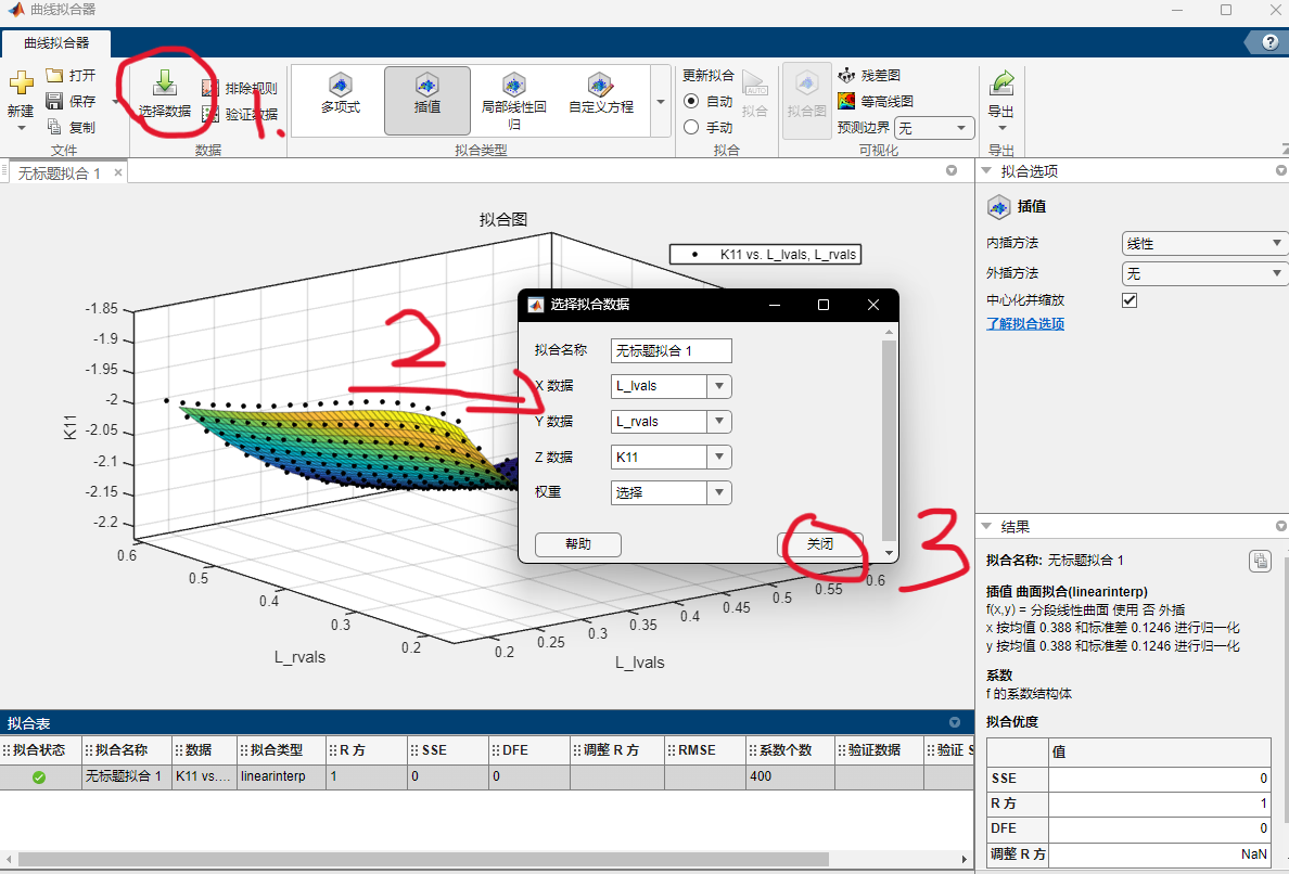
最上面一部分是对腿部质心,转动惯量等与腿长关系所拟合出的直线(一元一次方程),后面的 K 的拟合是利用 matlab 工具集 Curve Fitting Box 来做的。但是这个好像不能引用矩阵里面的某一块,只能直接引用一整个矩阵,所以才有了后面的一大段冗长的代码。
在 主页-附加功能 搜索这个工具集并且下载,然后在 APP 这个界面就会有这个曲线拟合器
加载数据,并且选择对应的数据,这里的话,如果只有两个变量,y 是因变量,而三个变量的话 z 就是因变量,x 和 y 就是自变量,权重不需选择
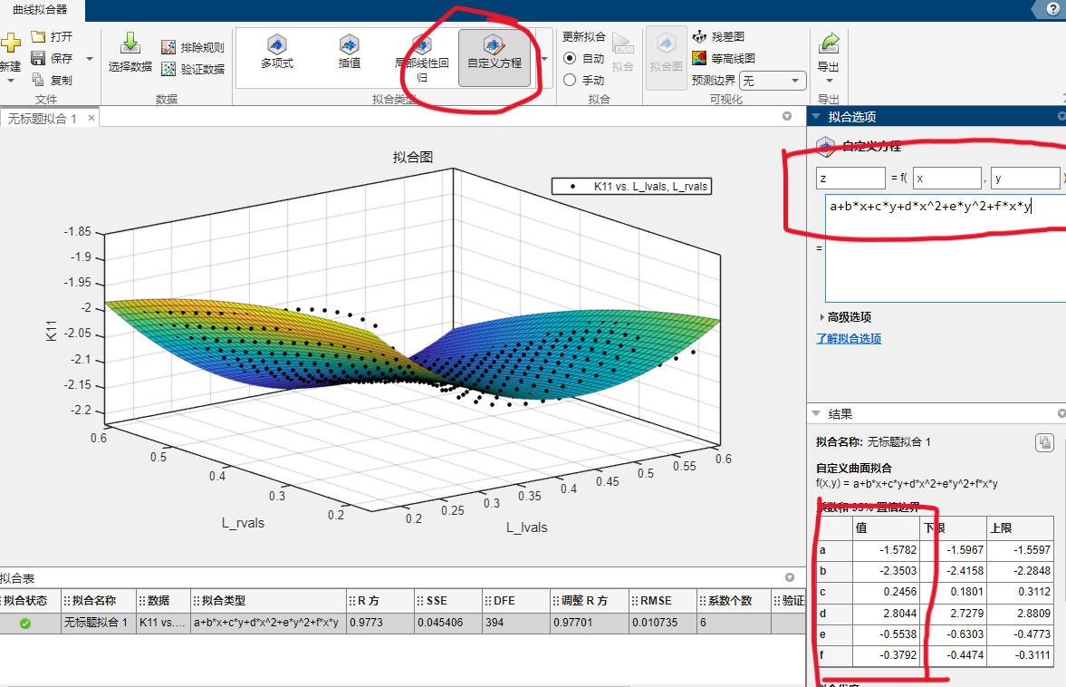
选择自定义方程,最后拟合得到的参数就是函数的系数(右下角)
有一点不太好的是,一次只能拟合一个 K 的系数,但是还是挺简单的,而且很直观,能很清楚的看到数据的拟合情况。
最后将这些数据写入代码中就可以了,需要注意的是 u = − K x u=-Kx u = − K x
控制器小结
半身控制器
比较简单,参数也比较少,但是必须要写 PID 来实现对机体整体的控制。左右两侧的身体都需要一个单独的半身控制器来进行控制,需要额外的 PID
腿部控制腿长 PID:输入当前腿长,目标腿长。输出为虚拟力。注意需要加一个前馈力,用以补偿重力和侧向惯性力矩
转向 PID:对于上述所得到的 LQR 控制器,发现并没有关于转向的 PID,所以需要自己写一个,输入就是当前转角,目标为目标角度,输出就是 Tw 的增益。注意方向
双腿夹角 PID:由于转向 PID 会影响左右轮子上的力矩,导致力矩不平衡,这就容易导致双腿劈叉,所以用双腿夹角 PID 来避免,最终输出结果叠加在 LQR 计算出的关节力矩上
全身控制器
比较复杂,系统状态空间方程会很难解算,只能说自己解了好久(2天,对应上面的半身控制器只用了一个小时),参数巨多,最终拟合出来的 K 的函数至少有 240 个参数,我只能说太魔鬼了。但是实际控制效果还是很不错的,需要的额外 PID 并不是很多
腿部控制腿长 PID:输入当前腿长,目标腿长。输出为虚拟力。注意需要加一个前馈力,用以补偿重力和侧向惯性力矩
比较
全身控制器相比半身控制器会更复杂,但是对系统的控制效果说实话还是很不错的,感觉控制的很细腻(不知道是不是好不容易解出来之后对自己的安慰)。可以都试试。
对于 ADRC 和 Hinfinty 控制器,并不是很好用,ADRC 来说,需要调试的参数太多,而且系统耦合性太强了,很不好调,而且也很复杂,主要是编程要写的太多了(doge)。Hinfinty 来说,也不需要调节参数,实际上只有一个 γ \gamma γ
但是不管怎么说,LQR 还算是一个不错的控制器的
在仿真中测试,整体上的控制是比单边控制要有更高的上限,并且对机体的控制确实更好
五连杆正运动学解算
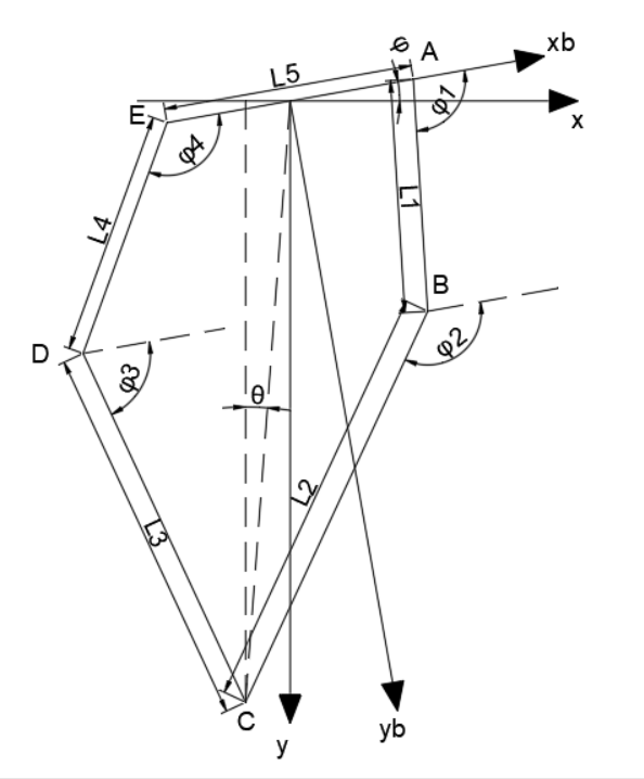
以杆 L 5 L_5 L 5 y b − x b y_b-x_b y b − x b y − x y-x y − x y b − x b y_b-x_b y b − x b
A = ( L 5 2 , 0 ) B = ( L 5 2 + L 1 cos φ 1 , L 1 sin φ 1 ) D = ( − L 5 2 + L 4 cos φ 4 , L 4 sin φ 4 ) E = ( − L 5 2 , 0 ) A=(\frac{L_5}{2}, 0)\\B=(\frac{L_5}{2}+L_1\cos\varphi_1,L_1\sin\varphi_1)\\D=(-\frac{L_5}{2}+L_4\cos\varphi_4,L_4\sin\varphi_4)\\E=(-\frac{L_5}{2},0)
A = ( 2 L 5 , 0 ) B = ( 2 L 5 + L 1 cos φ 1 , L 1 sin φ 1 ) D = ( − 2 L 5 + L 4 cos φ 4 , L 4 sin φ 4 ) E = ( − 2 L 5 , 0 )
通过五连杆左右两部分列写 C 点坐标,可以得到下列等式
{ B x + L 2 cos φ 2 = D x + L 3 cos φ 3 B y + L 2 sin φ 2 = D y + L 3 sin φ 3 \left\{\begin{aligned}&B_x+L_2\cos\varphi_2=D_x+L_3\cos\varphi_3\\&B_y+L_2\sin\varphi_2=D_y+L_3\sin\varphi_3\end{aligned}\right.
{ B x + L 2 cos φ 2 = D x + L 3 cos φ 3 B y + L 2 sin φ 2 = D y + L 3 sin φ 3
将两边进行平方
{ ( B x − D x ) 2 + 2 ( B x − D x ) L 2 cos ( φ 2 ) + L 2 2 cos 2 ( φ 2 ) = L 3 2 cos 2 φ 3 ( B y − D y ) 2 + 2 ( B y − D y ) L 2 sin ( φ 2 ) + L 2 2 sin 2 ( φ 2 ) = L 3 2 sin 2 φ 3 \left\{\begin{aligned}&(B_x-D_x)^2+2(B_x-D_x)L_2\cos(\varphi_2)+L_2^2\cos^2(\varphi_2)=L_3^2\cos^2\varphi_3\\&(B_y-D_y)^2+2(B_y-D_y)L_2\sin(\varphi_2)+L_2^2\sin^2(\varphi_2)=L_3^2\sin^2\varphi_3\end{aligned}\right.
{ ( B x − D x ) 2 + 2 ( B x − D x ) L 2 cos ( φ 2 ) + L 2 2 cos 2 ( φ 2 ) = L 3 2 cos 2 φ 3 ( B y − D y ) 2 + 2 ( B y − D y ) L 2 sin ( φ 2 ) + L 2 2 sin 2 ( φ 2 ) = L 3 2 sin 2 φ 3
两式相加得到
A cos φ 2 + B sin φ 2 + C = 0 A\cos\varphi_2+B\sin\varphi_2+C=0
A cos φ 2 + B sin φ 2 + C = 0
其中
A = 2 L 2 ( B x − D x ) B = 2 L 2 ( B y − D y ) L B D = ( B x − D x ) 2 + ( B y − D y ) 2 C = L 2 2 + L B D 2 − L 3 2 D = L 3 2 + L B D 2 − L 2 2 A=2L_2(B_x-D_x)\\B=2L_2(B_y-D_y)\\L_{BD}=\sqrt{(B_x-D_x)^2+(B_y-D_y)^2}\\C=L_2^2+L_{BD}^2-L_3^2\\D=L_3^2+L_{BD}^2-L_2^2
A = 2 L 2 ( B x − D x ) B = 2 L 2 ( B y − D y ) L B D = ( B x − D x ) 2 + ( B y − D y ) 2 C = L 2 2 + L B D 2 − L 3 2 D = L 3 2 + L B D 2 − L 2 2
利用倍角公式进行化简,此处用到的倍角公式为
tan φ 2 = sin φ 1 + cos φ \tan\frac{\varphi}{2}=\frac{\sin\varphi}{1+\cos\varphi}
tan 2 φ = 1 + cos φ sin φ
化简过程如下
1 + cos φ 2 2 ( 2 A cos φ 2 + 2 B sin φ 2 + 2 C 1 + cos φ 2 ) = 0 \frac{1+\cos\varphi_2}{2}(\frac{2A\cos\varphi_2+2B\sin\varphi_2+2C}{1+\cos\varphi_2})=0
2 1 + cos φ 2 ( 1 + cos φ 2 2 A cos φ 2 + 2 B sin φ 2 + 2 C ) = 0
将 2 A cos φ 2 2A\cos\varphi_2 2 A cos φ 2 2 C 2C 2 C
2 A cos φ 2 = A + cos φ 2 A − A + cos φ 2 A 2 C = C + cos φ 2 C + C − cos φ 2 C 2A\cos\varphi_2=A+\cos\varphi_2A-A+\cos\varphi_2A\\2C=C+\cos\varphi_2C+C-\cos\varphi_2C
2 A cos φ 2 = A + cos φ 2 A − A + cos φ 2 A 2 C = C + cos φ 2 C + C − cos φ 2 C
将上面两个公式化简为
2 A cos φ 2 + 2 C = ( A + C ) ( 1 + cos φ 2 ) + ( C − A ) ( 1 − cos φ 2 ) 2A\cos\varphi_2+2C=(A+C)(1+\cos\varphi_2)+(C-A)(1-\cos\varphi_2)
2 A cos φ 2 + 2 C = ( A + C ) ( 1 + cos φ 2 ) + ( C − A ) ( 1 − cos φ 2 )
所以上述公式可以化简为
1 + cos φ 2 2 ( 2 B sin φ 2 1 + cos φ 2 + ( A + C ) + ( C − A ) ( 1 − cos φ 2 ) 1 + cos φ 2 ) = 0 \frac{1+\cos\varphi_2}{2}\Big(\frac{2B\sin\varphi_2}{1+\cos\varphi_2}+(A+C)+\frac{(C-A)(1-\cos\varphi_2)}{1+\cos\varphi_2}\Big)=0
2 1 + cos φ 2 ( 1 + cos φ 2 2 B sin φ 2 + ( A + C ) + 1 + cos φ 2 ( C − A ) ( 1 − cos φ 2 ) ) = 0
其中第三项可以化简为
( C − A ) ( 1 − cos φ 2 ) 1 + cos φ 2 = ( C − A ) sin 2 φ 2 ( 1 + cos φ 2 ) 2 \frac{(C-A)(1-\cos\varphi_2)}{1+\cos\varphi_2}=\frac{(C-A)\sin^2\varphi_2}{(1+\cos\varphi_2)^2}
1 + cos φ 2 ( C − A ) ( 1 − cos φ 2 ) = ( 1 + cos φ 2 ) 2 ( C − A ) sin 2 φ 2
所以公式可以化简为
( C − A ) tan 2 φ 2 2 + 2 B tan φ 2 2 + ( A + C ) = 0 (C-A)\tan^2\frac{\varphi_2}{2}+2B\tan\frac{\varphi_2}{2}+(A+C)=0
( C − A ) tan 2 2 φ 2 + 2 B tan 2 φ 2 + ( A + C ) = 0
可以求解这个一元二次方程,得到
φ 2 = 2 arctan ( − B ± B 2 − C 2 + A 2 C − A ) φ 3 = 2 arctan ( B ± B 2 − D 2 + A 2 D + A ) \varphi_2=2\arctan(\frac{-B\plusmn\sqrt{B^2-C^2+A^2}}{C-A})\\\varphi_3=2\arctan(\frac{B\plusmn\sqrt{B^2-D^2+A^2}}{D+A})
φ 2 = 2 arctan ( C − A − B ± B 2 − C 2 + A 2 ) φ 3 = 2 arctan ( D + A B ± B 2 − D 2 + A 2 )
这是有两个解的,当然连杆状态也是由两个解的,所以可以验算 φ 2 , φ 3 \varphi_2,\varphi_3 φ 2 , φ 3 sin φ 2 > 0 , sin φ 3 > 0 \sin\varphi_2>0,\sin\varphi_3>0 sin φ 2 > 0 , sin φ 3 > 0
C x = L 5 2 + L 1 cos ( φ 1 ) + L 2 cos ( φ 2 ) C y = L 1 sin ( φ 1 ) + L 2 sin ( φ 2 ) C_x=\frac{L_5}{2}+L_1\cos(\varphi_1)+L_2\cos(\varphi_2)\\C_y=L_1\sin(\varphi_1)+L_2\sin(\varphi_2)
C x = 2 L 5 + L 1 cos ( φ 1 ) + L 2 cos ( φ 2 ) C y = L 1 sin ( φ 1 ) + L 2 sin ( φ 2 )
从而得到在机体坐标系下的腿长 L L L φ 0 \varphi_0 φ 0
L 0 = C x 2 + C y 2 θ b = arctan C y C x L_0=\sqrt{C_x^2+C_y^2}\\\theta_b=\arctan\frac{C_y}{C_x}
L 0 = C x 2 + C y 2 θ b = arctan C x C y
将坐标映射到 y − x y-x y − x
[ C x ′ C y ′ ] = [ cos φ sin φ − sin φ cos φ ] [ C x C y ] \begin{bmatrix}C_x^\prime\\C_y^\prime\end{bmatrix}=\begin{bmatrix}\cos\varphi&\sin\varphi\\-\sin\varphi&\cos\varphi\end{bmatrix}\begin{bmatrix}C_x\\C_y\end{bmatrix}
[ C x ′ C y ′ ] = [ cos φ − sin φ sin φ cos φ ] [ C x C y ]
最终可以得到腿长 L L L θ \theta θ
L ′ = ( C x ′ ) 2 + ( C y ′ ) 2 θ ′ = arctan ( − C x ′ C y ′ ) L^\prime=\sqrt{(C_x^\prime)^2+(C_y^\prime)^2}\\\theta^\prime=\arctan(-\frac{C_x^\prime}{C_y^\prime})
L ′ = ( C x ′ ) 2 + ( C y ′ ) 2 θ ′ = arctan ( − C y ′ C x ′ )
VMC
作用是在每个需要控制的自由度上构造合适的虚拟构件来产生合适的虚拟力。虚拟力不是实际执行机构的作用力或力矩,而是通过执行机构的作用经过机构转换而成。对于一些控制问题,我们可能需要将工作空间 (Task Space) 的力或力矩映射成关节空间 (Joint Space) 的关节力矩
在五连杆中,需要获得机构末端沿腿的推力 F F F T b T_b T b L 0 , θ b L_0,\theta_b L 0 , θ b A , E A,E A , E T A , T E T_A,T_E T A , T E
x = [ L 0 θ b ] q = [ φ 1 φ 4 ] x=\begin{bmatrix}L_0\\\theta_b\end{bmatrix}\\q=\begin{bmatrix}\varphi_1\\\varphi_4\end{bmatrix}
x = [ L 0 θ b ] q = [ φ 1 φ 4 ]
对正运动学模型 x = f ( q ) x=f(q) x = f ( q )
f ′ = [ ∂ L 0 ∂ φ 1 ∂ L 0 ∂ φ 4 ∂ θ b ∂ φ 1 ∂ θ b ∂ φ 4 ] f'=\begin{bmatrix}\frac{\partial L_0}{\partial \varphi_1}&\frac{\partial L_0}{\partial \varphi_4}\\\frac{\partial \theta_b}{\partial \varphi_1}&\frac{\partial\theta_b}{\partial \varphi_4}\end{bmatrix}
f ′ = [ ∂ φ 1 ∂ L 0 ∂ φ 1 ∂ θ b ∂ φ 4 ∂ L 0 ∂ φ 4 ∂ θ b ]
这就是 x 对 q 的雅各比矩阵,记作 J J J
Δ x = J Δ q \Delta x=J\Delta q
Δ x = J Δ q
通过雅各比矩阵 J J J q ˙ \dot{q} q ˙ x ˙ \dot{x} x ˙
T T Δ q + ( − F ) T Δ x = 0 T = [ T A T E ] F p o l e = [ F T b ] T^T\Delta q+(-F)^T\Delta x=0\\T=\begin{bmatrix}T_A\\T_E\end{bmatrix}\\F_{pole}=\begin{bmatrix}F\\T_b\end{bmatrix}
T T Δ q + ( − F ) T Δ x = 0 T = [ T A T E ] F p o l e = [ F T b ]
将全微分方程带入之后可得
T = J T F p o l e T=J^TF_{pole}
T = J T F p o l e
但是上述推导中的正运动学模型直接求雅各比矩阵比较困难,因为模型中有大量的平方与三角函数的运算,结果比较复杂。所以进行改进,由于雅各比矩阵实际上描述的是两坐标微分的线性映射关系,所以可以计算速度映射来得到雅各比矩阵。由于 L 0 , φ 0 L_0,\varphi_0 L 0 , φ 0 C C C C C C
x ˙ C = − L 1 φ ˙ 1 sin φ 1 − L 2 φ ˙ 2 sin φ 2 y ˙ C = L 1 φ ˙ 1 cos φ 1 + L 2 φ ˙ 2 cos φ 2 \dot{x}_C=-L_1\dot{\varphi}_1\sin\varphi_1-L_2\dot{\varphi}_2\sin\varphi_2\\\dot{y}_C=L_1\dot{\varphi}_1\cos\varphi_1+L_2\dot{\varphi}_2\cos\varphi_2
x ˙ C = − L 1 φ ˙ 1 sin φ 1 − L 2 φ ˙ 2 sin φ 2 y ˙ C = L 1 φ ˙ 1 cos φ 1 + L 2 φ ˙ 2 cos φ 2
通过五连杆左右两部分列写 C 点坐标求导可以得到 φ ˙ 2 \dot\varphi_2 φ ˙ 2
{ x ˙ B − L 2 φ ˙ 2 sin φ 2 = x ˙ D − L 3 φ ˙ 3 sin φ 3 y B + L 2 sin φ 2 = y D + L 3 sin φ 3 \left\{\begin{aligned}&\dot x_B-L_2\dot\varphi_2\sin\varphi_2=\dot x_D-L_3\dot\varphi_3\sin\varphi_3\\&y_B+L_2\sin\varphi_2=y_D+L_3\sin\varphi_3\end{aligned}\right.
{ x ˙ B − L 2 φ ˙ 2 sin φ 2 = x ˙ D − L 3 φ ˙ 3 sin φ 3 y B + L 2 sin φ 2 = y D + L 3 sin φ 3
消去 φ ˙ 3 \dot\varphi_3 φ ˙ 3 φ ˙ 2 \dot\varphi_2 φ ˙ 2
φ ˙ 2 = ( x ˙ D − x ˙ B ) cos φ 3 + ( y ˙ D − y ˙ B ) sin φ 3 L 2 sin ( φ 3 − φ 2 ) \dot\varphi_2=\frac{(\dot x_D-\dot x_B)\cos\varphi_3+(\dot y_D-\dot y_B)\sin\varphi_3}{L_2\sin(\varphi_3-\varphi_2)}
φ ˙ 2 = L 2 sin ( φ 3 − φ 2 ) ( x ˙ D − x ˙ B ) cos φ 3 + ( y ˙ D − y ˙ B ) sin φ 3
其中
x ˙ B = − L 2 φ ˙ 1 sin φ 1 y ˙ B = L 2 φ ˙ 1 cos φ 1 x ˙ D = − L 4 φ ˙ 4 sin φ 4 y ˙ D = L 4 φ ˙ 4 sin φ 4 \dot x_B=-L_2\dot\varphi_1\sin\varphi_1\\\dot y_B=L_2\dot\varphi_1\cos\varphi_1\\\dot x_D=-L_4\dot\varphi_4\sin\varphi_4\\\dot y_D=L_4\dot\varphi_4\sin\varphi_4
x ˙ B = − L 2 φ ˙ 1 sin φ 1 y ˙ B = L 2 φ ˙ 1 cos φ 1 x ˙ D = − L 4 φ ˙ 4 sin φ 4 y ˙ D = L 4 φ ˙ 4 sin φ 4
并且其中的 φ ˙ 1 , φ ˙ 4 \dot\varphi_1,\dot\varphi_4 φ ˙ 1 , φ ˙ 4
x ˙ C = − L 1 φ ˙ 1 sin φ 1 − L 2 ( x ˙ D − x ˙ B ) cos φ 3 + ( y ˙ D − y ˙ B ) sin φ 3 L 2 sin ( φ 3 − φ 2 ) sin φ 2 y ˙ C = L 1 φ ˙ 1 cos φ 1 + L 2 ( x ˙ D − x ˙ B ) cos φ 3 + ( y ˙ D − y ˙ B ) sin φ 3 L 2 sin ( φ 3 − φ 2 ) cos φ 2 \dot{x}_C=-L_1\dot{\varphi}_1\sin\varphi_1-L_2\frac{(\dot x_D-\dot x_B)\cos\varphi_3+(\dot y_D-\dot y_B)\sin\varphi_3}{L_2\sin(\varphi_3-\varphi_2)}\sin\varphi_2\\\dot{y}_C=L_1\dot{\varphi}_1\cos\varphi_1+L_2\frac{(\dot x_D-\dot x_B)\cos\varphi_3+(\dot y_D-\dot y_B)\sin\varphi_3}{L_2\sin(\varphi_3-\varphi_2)}\cos\varphi_2
x ˙ C = − L 1 φ ˙ 1 sin φ 1 − L 2 L 2 sin ( φ 3 − φ 2 ) ( x ˙ D − x ˙ B ) cos φ 3 + ( y ˙ D − y ˙ B ) sin φ 3 sin φ 2 y ˙ C = L 1 φ ˙ 1 cos φ 1 + L 2 L 2 sin ( φ 3 − φ 2 ) ( x ˙ D − x ˙ B ) cos φ 3 + ( y ˙ D − y ˙ B ) sin φ 3 cos φ 2
化简之后得到
[ x ˙ C y ˙ C ] = [ L 1 sin ( φ 1 − φ 2 ) sin φ 3 sin ( φ 2 − φ 3 ) L 4 sin ( φ 3 − φ 4 ) sin φ 2 sin ( φ 2 − φ 3 ) − L 1 sin ( φ 1 − φ 2 ) cos φ 3 sin ( φ 2 − φ 3 ) − L 4 sin ( φ 3 − φ 4 ) cos φ 2 sin ( φ 2 − φ 3 ) ] [ φ ˙ 1 φ ˙ 4 ] \begin{bmatrix}\dot x_C\\\dot y_C\end{bmatrix}=\begin{bmatrix}\frac{L_1\sin(\varphi_1-\varphi_2)\sin\varphi_3}{\sin(\varphi_2-\varphi_3)}&\frac{L_4\sin(\varphi_3-\varphi_4)\sin\varphi_2}{\sin(\varphi_2-\varphi_3)}\\-\frac{L_1\sin(\varphi_1-\varphi_2)\cos\varphi_3}{\sin(\varphi_2-\varphi_3)}&-\frac{L_4\sin(\varphi_3-\varphi_4)\cos\varphi_2}{\sin(\varphi_2-\varphi_3)}\end{bmatrix}\begin{bmatrix}\dot \varphi_1\\\dot \varphi_4\end{bmatrix}
[ x ˙ C y ˙ C ] = [ s i n ( φ 2 − φ 3 ) L 1 s i n ( φ 1 − φ 2 ) s i n φ 3 − s i n ( φ 2 − φ 3 ) L 1 s i n ( φ 1 − φ 2 ) c o s φ 3 s i n ( φ 2 − φ 3 ) L 4 s i n ( φ 3 − φ 4 ) s i n φ 2 − s i n ( φ 2 − φ 3 ) L 4 s i n ( φ 3 − φ 4 ) c o s φ 2 ] [ φ ˙ 1 φ ˙ 4 ]
记作
[ x ˙ C y ˙ C ] = J [ φ ˙ 1 φ ˙ 4 ] \begin{bmatrix}\dot x_C\\\dot y_C\end{bmatrix}=J\begin{bmatrix}\dot \varphi_1\\\dot \varphi_4\end{bmatrix}
[ x ˙ C y ˙ C ] = J [ φ ˙ 1 φ ˙ 4 ]
由于速度雅各比矩阵是力矩雅各比矩阵的转置,则上述可以得到关节力矩 T T T
T = J T [ F x F y ] [ F x F y ] = [ cos θ b − sin θ b L b sin θ b cos θ b L b ] [ F T b ] T=J^T\begin{bmatrix}F_x\\F_y\end{bmatrix}\\\begin{bmatrix}F_x\\F_y\end{bmatrix}=\begin{bmatrix}\cos\theta_b&-\frac{\sin\theta_b}{L_b}\\\sin\theta_b&\frac{\cos\theta_b}{L_b}\end{bmatrix}\begin{bmatrix}F\\T_b\end{bmatrix}
T = J T [ F x F y ] [ F x F y ] = [ cos θ b sin θ b − L b s i n θ b L b c o s θ b ] [ F T b ]
依次带入得到最终的关节力矩与虚拟力之间的映射关系
T = J T [ cos θ b − sin θ b L b sin θ b cos θ b L b ] [ F T b ] T=J^T\begin{bmatrix}\cos\theta_b&-\frac{\sin\theta_b}{L_b}\\\sin\theta_b&\frac{\cos\theta_b}{L_b}\end{bmatrix}\begin{bmatrix}F\\T_b\end{bmatrix}
T = J T [ cos θ b sin θ b − L b s i n θ b L b c o s θ b ] [ F T b ]
令
A = L 1 sin ( φ 1 − φ 2 ) sin ( φ 2 − φ 3 ) B = L 4 sin ( φ 3 − φ 4 ) sin ( φ 2 − φ 3 ) A=\frac{L_1\sin(\varphi_1-\varphi_2)}{\sin(\varphi_2-\varphi_3)}\\B=\frac{L_4\sin(\varphi_3-\varphi_4)}{\sin(\varphi_2-\varphi_3)}
A = sin ( φ 2 − φ 3 ) L 1 sin ( φ 1 − φ 2 ) B = sin ( φ 2 − φ 3 ) L 4 sin ( φ 3 − φ 4 )
最终带入得到
T = [ A sin ( φ 3 − θ b ) − A cos ( φ 3 − θ b ) L b B sin ( φ 2 − θ b ) − B cos ( φ 2 − θ b ) L b ] F p o l e T=\begin{bmatrix}A\sin(\varphi_3-\theta_b)&-\frac{A\cos(\varphi_3-\theta_b)}{L_b}\\B\sin(\varphi_2-\theta_b)&-\frac{B\cos(\varphi_2-\theta_b)}{L_b}\end{bmatrix}F_{pole}
T = [ A sin ( φ 3 − θ b ) B sin ( φ 2 − θ b ) − L b A c o s ( φ 3 − θ b ) − L b B c o s ( φ 2 − θ b ) ] F p o l e
反向 VMC 如下
F p o l e = [ − cos ( φ 2 − θ b ) L 1 sin ( φ 1 − φ 2 ) cos ( φ 3 − θ b ) L 4 sin ( φ 3 − φ 4 ) − L b sin ( φ 2 − θ b ) L 1 sin ( φ 1 − φ 2 ) L b sin ( φ 3 − θ b ) L 4 sin ( φ 3 − φ 4 ) ] T F_{pole}=\begin{bmatrix}\frac{-\cos(\varphi_2-\theta_b)}{L_1\sin(\varphi_1-\varphi_2)}&\frac{\cos(\varphi_3-\theta_b)}{L_4\sin(\varphi_3-\varphi_4)}\\-\frac{L_b\sin(\varphi_2-\theta_b)}{L_1\sin(\varphi_1-\varphi_2)}&\frac{L_b\sin(\varphi_3-\theta_b)}{L_4\sin(\varphi_3-\varphi_4)}\end{bmatrix}T
F p o l e = [ L 1 s i n ( φ 1 − φ 2 ) − c o s ( φ 2 − θ b ) − L 1 s i n ( φ 1 − φ 2 ) L b s i n ( φ 2 − θ b ) L 4 s i n ( φ 3 − φ 4 ) c o s ( φ 3 − θ b ) L 4 s i n ( φ 3 − φ 4 ) L b s i n ( φ 3 − θ b ) ] T
腿部摆角补偿
在腿部结构上,连杆结构的前后分布并不均匀,所以需要一个 θ \theta θ θ \theta θ θ \theta θ
首先在机器人坐标系 x b − y b x_b-y_b x b − y b
Z b = [ c x − c y ] Z l 1 = [ l 5 2 + l 1 b cos φ 1 l 1 b sin φ 1 ] Z l 2 = [ l 5 2 + l 1 cos φ 1 + l 2 b cos φ 2 l 1 sin φ 1 + l 2 b sin φ 2 ] Z l 3 = [ − l 5 2 + l 4 cos φ 4 + l 3 b cos φ 3 l 4 sin φ 4 + l 3 b sin φ 3 ] Z l 4 = [ − l 5 2 + l 4 b cos φ 4 l 4 b sin φ 4 ] Z_b=\begin{bmatrix}c_x\\-c_y\end{bmatrix}\\Z_{l_1}=\begin{bmatrix}\frac{l_5}{2}+l_{1b}\cos\varphi_1\\l_{1b}\sin\varphi_1\end{bmatrix}\\Z_{l_2}=\begin{bmatrix}\frac{l_5}{2}+l_1\cos\varphi_1+l_{2b}\cos\varphi_2\\l_1\sin\varphi_1+l_{2b}\sin\varphi_2\end{bmatrix}\\Z_{l_3}=\begin{bmatrix}-\frac{l_5}{2}+l_4\cos\varphi_4+l_{3b}\cos\varphi_3\\l_4\sin\varphi_4+l_{3b}\sin\varphi_3\end{bmatrix}\\Z_{l_4}=\begin{bmatrix}-\frac{l_5}{2}+l_{4b}\cos\varphi_4\\l_{4b}\sin\varphi_4\end{bmatrix}
Z b = [ c x − c y ] Z l 1 = [ 2 l 5 + l 1 b cos φ 1 l 1 b sin φ 1 ] Z l 2 = [ 2 l 5 + l 1 cos φ 1 + l 2 b cos φ 2 l 1 sin φ 1 + l 2 b sin φ 2 ] Z l 3 = [ − 2 l 5 + l 4 cos φ 4 + l 3 b cos φ 3 l 4 sin φ 4 + l 3 b sin φ 3 ] Z l 4 = [ − 2 l 5 + l 4 b cos φ 4 l 4 b sin φ 4 ]
将重心坐标系转移到轮子坐标系 x w − y w x_w-y_w x w − y w
Z b = [ cos φ sin φ − sin φ cos φ ] [ c x − c y ] + [ L sin θ c − L cos θ c ] Z l 1 = [ cos φ sin φ − sin φ cos φ ] [ l 5 2 + l 1 b cos φ 1 l 1 b sin φ 1 ] + [ L sin θ c − L cos θ c ] Z l 2 = [ cos φ sin φ − sin φ cos φ ] [ l 5 2 + l 1 cos φ 1 + l 2 b cos φ 2 l 1 sin φ 1 + l 2 b sin φ 2 ] + [ L sin θ c − L cos θ c ] Z l 3 = [ cos φ sin φ − sin φ cos φ ] [ − l 5 2 + l 4 cos φ 4 + l 3 b cos φ 3 l 4 sin φ 4 + l 3 b sin φ 3 ] + [ L sin θ c − L cos θ c ] Z l 4 = [ cos φ sin φ − sin φ cos φ ] [ − l 5 2 + l 4 b cos φ 4 l 4 b sin φ 4 ] + [ L sin θ c − L cos θ c ] Z_b=\begin{bmatrix}\cos\varphi&\sin\varphi\\-\sin\varphi&\cos\varphi\end{bmatrix}\begin{bmatrix}c_x\\-c_y\end{bmatrix}+\begin{bmatrix}L\sin\theta_c\\-L\cos\theta_c\end{bmatrix}\\Z_{l_1}=\begin{bmatrix}\cos\varphi&\sin\varphi\\-\sin\varphi&\cos\varphi\end{bmatrix}\begin{bmatrix}\frac{l_5}{2}+l_{1b}\cos\varphi_1\\l_{1b}\sin\varphi_1\end{bmatrix}+\begin{bmatrix}L\sin\theta_c\\-L\cos\theta_c\end{bmatrix}\\Z_{l_2}=\begin{bmatrix}\cos\varphi&\sin\varphi\\-\sin\varphi&\cos\varphi\end{bmatrix}\begin{bmatrix}\frac{l_5}{2}+l_1\cos\varphi_1+l_{2b}\cos\varphi_2\\l_1\sin\varphi_1+l_{2b}\sin\varphi_2\end{bmatrix}+\begin{bmatrix}L\sin\theta_c\\-L\cos\theta_c\end{bmatrix}\\Z_{l_3}=\begin{bmatrix}\cos\varphi&\sin\varphi\\-\sin\varphi&\cos\varphi\end{bmatrix}\begin{bmatrix}-\frac{l_5}{2}+l_4\cos\varphi_4+l_{3b}\cos\varphi_3\\l_4\sin\varphi_4+l_{3b}\sin\varphi_3\end{bmatrix}+\begin{bmatrix}L\sin\theta_c\\-L\cos\theta_c\end{bmatrix}\\Z_{l_4}=\begin{bmatrix}\cos\varphi&\sin\varphi\\-\sin\varphi&\cos\varphi\end{bmatrix}\begin{bmatrix}-\frac{l_5}{2}+l_{4b}\cos\varphi_4\\l_{4b}\sin\varphi_4\end{bmatrix}+\begin{bmatrix}L\sin\theta_c\\-L\cos\theta_c\end{bmatrix}
Z b = [ cos φ − sin φ sin φ cos φ ] [ c x − c y ] + [ L sin θ c − L cos θ c ] Z l 1 = [ cos φ − sin φ sin φ cos φ ] [ 2 l 5 + l 1 b cos φ 1 l 1 b sin φ 1 ] + [ L sin θ c − L cos θ c ] Z l 2 = [ cos φ − sin φ sin φ cos φ ] [ 2 l 5 + l 1 cos φ 1 + l 2 b cos φ 2 l 1 sin φ 1 + l 2 b sin φ 2 ] + [ L sin θ c − L cos θ c ] Z l 3 = [ cos φ − sin φ sin φ cos φ ] [ − 2 l 5 + l 4 cos φ 4 + l 3 b cos φ 3 l 4 sin φ 4 + l 3 b sin φ 3 ] + [ L sin θ c − L cos θ c ] Z l 4 = [ cos φ − sin φ sin φ cos φ ] [ − 2 l 5 + l 4 b cos φ 4 l 4 b sin φ 4 ] + [ L sin θ c − L cos θ c ]
假定此时的 θ c \theta_c θ c
M Z b x + m 1 Z l 1 x + m 2 Z l 2 x + m 3 Z l 3 x + m 4 Z l 4 x = 0 MZ_{bx}+m_1Z_{l_1x}+m_2Z_{l_2x}+m_3Z_{l_3x}+m_4Z_{l_4x}=0
M Z b x + m 1 Z l 1 x + m 2 Z l 2 x + m 3 Z l 3 x + m 4 Z l 4 x = 0
求解可以得到 θ \theta θ
θ = − arcsin ( l 5 ( m 1 + m 2 − m 3 − m 4 ) + 2 M c x ) cos ( φ ) − 2 M c y sin ( φ ) + 2 ( l 1 m 2 + l 1 b m 1 ) cos ( φ − φ 1 ) + 2 l 2 b m 2 cos ( φ − φ 2 ) + 2 l 3 b m 3 cos ( φ − φ 3 ) + 2 ( l 4 m 3 + l 4 b m 4 ) cos ( φ − φ 4 ) 2 L ( M + m 1 + m 2 + m 3 + m 4 ) \theta=-\arcsin\frac{\Big(l_5(m_1+m_2-m_3-m_4)+2Mc_x\Big)\cos(\varphi)-2Mc_y\sin(\varphi)+2(l_1m_2+l_{1b}m_1)\cos(\varphi-\varphi_1)+2l_{2b}m_2\cos(\varphi-\varphi_2)+2l_{3b}m_3\cos(\varphi-\varphi_3)+2(l_4m_3+l_{4b}m_4)\cos(\varphi-\varphi_4)}{2L(M+m_1+m_2+m_3+m_4)}
θ = − arcsin 2 L ( M + m 1 + m 2 + m 3 + m 4 ) ( l 5 ( m 1 + m 2 − m 3 − m 4 ) + 2 M c x ) cos ( φ ) − 2 M c y sin ( φ ) + 2 ( l 1 m 2 + l 1 b m 1 ) cos ( φ − φ 1 ) + 2 l 2 b m 2 cos ( φ − φ 2 ) + 2 l 3 b m 3 cos ( φ − φ 3 ) + 2 ( l 4 m 3 + l 4 b m 4 ) cos ( φ − φ 4 )
在使用时可以直接添加到当前状态中,即状态空间方程变为
X = [ θ − θ c θ ˙ x x ˙ φ φ ˙ ] X=\begin{bmatrix}\theta-\theta_c\\\dot{\theta}\\x\\\dot{x}\\\varphi\\\dot\varphi\end{bmatrix}
X = ⎣ ⎢ ⎢ ⎢ ⎢ ⎢ ⎢ ⎢ ⎡ θ − θ c θ ˙ x x ˙ φ φ ˙ ⎦ ⎥ ⎥ ⎥ ⎥ ⎥ ⎥ ⎥ ⎤
腿长控制
腿长控制是直接使用 PID 进行控制,但是一定要将控制腿长的 PID 调节的软一点,P 要小一点,D 要尽量小,I 尽量不给。需要保证腿最长的时候能够平衡前馈力和轮子的重力从而有向上拉的力,而腿长最短时保证腿部力能支撑起整个机体。最终 PID 的输出与前馈力之和作为腿部的沿杆的力参与 VMC 解算
腿长 PID 较大会造成很大的影响,PID 过大导致系统的控制腿长的输出太大,相对应的控制整个系统的平衡的输出就很小,从而导致系统稳定性不够
例如:电机的输出的力矩是有限的,当把 LQR + VMC 解算出来的力矩同腿长控制 PID 的输出相结合之后,就会比较大,那么进行力矩限制时,会导致限制之后的力矩不能保证机体平衡或者腿长的控制,最终控制效果不好
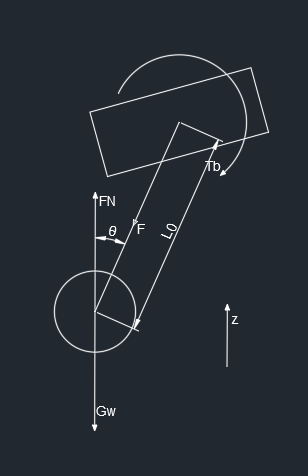
离地检测
根据图中可以得到
m w z ¨ w = F N − F cos θ + T b sin θ L 0 m_w\ddot{z}_w=F_N-F\cos\theta+\frac{T_b\sin\theta}{L_0}
m w z ¨ w = F N − F cos θ + L 0 T b sin θ
其中
z w = z b − L 0 cos θ ⇓ z ¨ w = z ¨ b − L ¨ 0 cos θ + 2 L ˙ 0 θ ˙ sin θ + L 0 θ ¨ sin θ + L 0 θ ˙ 2 cos θ z_w=z_b-L_0\cos\theta\\\\
\Downarrow\\\\
\ddot{z}_w=\ddot{z}_b-\ddot{L}_0\cos\theta+2\dot{L}_0\dot{\theta}\sin\theta+L_0\ddot{\theta}\sin\theta+L_0\dot{\theta}^2\cos\theta
z w = z b − L 0 cos θ ⇓ z ¨ w = z ¨ b − L ¨ 0 cos θ + 2 L ˙ 0 θ ˙ sin θ + L 0 θ ¨ sin θ + L 0 θ ˙ 2 cos θ
并且其中的 z ¨ b \ddot{z}_b z ¨ b
z ¨ b = ( a z cos φ + a x sin φ ) cos γ + a y sin γ \ddot{z}_b=(a_z\cos\varphi+a_x\sin\varphi)\cos{\gamma}+a_y\sin\gamma
z ¨ b = ( a z cos φ + a x sin φ ) cos γ + a y sin γ
并且 F F F T b T_b T b
( J T R M ) − 1 T = F p o l e (J^TRM)^{-1}T=F_{pole}
( J T R M ) − 1 T = F p o l e
得到
F N = m w ( z ¨ b − L ¨ 0 cos θ + 2 L ˙ 0 θ ˙ sin θ + L 0 θ ¨ sin θ + L 0 θ ˙ 2 cos θ ) + F cos θ − T b sin θ L 0 F_N=m_w(\ddot{z}_b-\ddot{L}_0\cos\theta+2\dot{L}_0\dot{\theta}\sin\theta+L_0\ddot{\theta}\sin\theta+L_0\dot{\theta}^2\cos\theta)+F\cos\theta-\frac{T_b\sin\theta}{L_0}
F N = m w ( z ¨ b − L ¨ 0 cos θ + 2 L ˙ 0 θ ˙ sin θ + L 0 θ ¨ sin θ + L 0 θ ˙ 2 cos θ ) + F cos θ − L 0 T b sin θ
可以判断,当 F N F_N F N θ , θ ˙ \theta,\dot\theta θ , θ ˙
1
2
3
4
5
6
7
8
9
10
11
float A = l1 * sin (angle1 - angle2) / sin (angle2 - angle3);float B = l4 * sin (angle3 - angle4) / sin (angle2 - angle3);A = A * cos (angle2 + theta.now) * sin (angle3 + theta.now) - A * cos (angle3 + theta.now) * sin (angle2 + theta.now); B = B * cos (angle2 + theta.now) * sin (angle3 + theta.now) - B * cos (angle3 + theta.now) * sin (angle2 + theta.now); Eigen::Matrix<float , 2 , 2 > trans; trans << sin (angle2 + theta.now) / A, -sin (angle3 + theta.now) / B, L0.now * cos (angle2 + theta.now) / B, -L0.now * cos (angle3 + theta.now) / B; Fnow = -trans(0 , 0 ) * jointF->torqueRead - trans(0 , 1 ) * jointB->torqueRead; Tbnow = -trans(1 , 0 ) * jointF->torqueRead - trans(1 , 1 ) * jointB->torqueRead;
最终得到
F N = F l , n o w + F r , n o w 2 F_N = \frac{F_{l,now} + F_{r,now}}{2}
F N = 2 F l , n o w + F r , n o w
跳跃控制
有些轮腿的控制中,是直接给一个比较大的力矩来使得机体跳跃,但是这样的话感觉并不是很好。所以有另一种方法:通过设定腿部杆长伸腿和蹬腿来实现跳跃
具体的腿部运动流程就是:收腿 → \rightarrow → → \rightarrow → → \rightarrow →
1
2
3
4
5
6
7
8
9
10
11
12
13
14
15
16
17
18
19
20
21
22
23
24
25
26
27
28
29
30
switch (jump_process) { case 1 : leg_len_l_set = min_leg_len; leg_len_r_set = min_leg_len; if (fabsf(leg_len_l_set - min_leg_len) < 0.01f && fabsf(leg_len_r_set - min_leg_len) < 0.01f ) ++jump_process; break ; case 2 : leg_len_l_set = max_leg_len; leg_len_r_set = max_leg_len; if (fabsf(leg_len_l_set - max_leg_len) < 0.01f && fabsf(leg_len_r_set - max_leg_len) < 0.01f ) ++jump_process; break ; case 3 : leg_len_l_set = min_leg_len; leg_len_r_set = min_leg_len; if (fabsf(leg_len_l_set - min_leg_len) < 0.01f && fabsf(leg_len_r_set - min_leg_len) < 0.01f ) ++jump_process; break ; case 4 : leg_len_l_set = buffer_leg_len; leg_len_r_set = buffer_leg_len; if (fabsf(leg_len_l_set - buffer_leg_len) < 0.01f && fabsf(leg_len_r_set - buffer_leg_len) < 0.01f ) ++jump_process; break ; default : break ; }
转角控制
转角可以直接利用 PID 进行控制,可以实现比较准确的控制,但是一般来说,这个 PID 的参数应当是一个 PD 控制器,这会保证系统不会因为卡住而出现大电流
由于机体的转角是受到轮子的差速转动实现的,所以 PID 的输出结果需要叠加到轮子的输出力矩上。但是如果转角比较大时,叠加到轮子的输出力矩上之后,左右两侧的机体可能出现运动不一致而导致机体发生劈叉等情况,所以还需要双腿角度 PID,用以防止双腿劈叉
横滚角控制
直接根据当前的横滚角,计算当机体保持平衡的时候两条腿的长度之差,然后叠加在当前腿长上,作为设定腿长来给左右两条腿进行控制
1
2
3
float leg_dif = sin (roll) * l_body;leg_len_l_set -= leg_dir / 2 ; leg_len_r_set += leg_dir / 2 ;
后记
整个控制系统是断断续续的研究了很久才能实现,这个机器人的控制确实很难,对于菜鸟的我来说确实很痛苦,但是研究出来之后会发现,原来当时困扰自己的东西只是一些小问题
实际上是做了两代轮腿,第一代死于经验不足,调试了差不多一个月然后被去安排做其他事情了。然后第二代轮腿实际上只在 4 天就成功了(喜极而泣),其实就是因为对其原理的理解不够清晰(一直觉得是机械结构设计不好,其实应该是我的问题)
再者即使调不出来也别放弃,重新整理一下思路,总会发现不一样的东西的